Initial look at Environmental Data
Received environmental data from the 2016 DNR outplant today. Plotted and ran some stats in thie R Script
I checked out mean, standard deviation and variance for each measurement across treatments:
| Stat | WBE | WBB | SKE | SKB | PGE | PGB | CIE | CIB | FBE | FBB | |———|———|———|———|———|———|———|———|———|———|———| | pH-Mean | 7.8091 | 7.6086 | 7.5225 | 7.3927 | NA | 7.4155 | 7.9116 | 7.7109 | 7.9003 | 7.4598 | | pH-SD | 0.0946 | 0.1871 | 0.2824 | 0.2533 | NA | 0.2432 | 0.1793 | 0.2663 | 0.1947 | 0.2328 | | pH-Var | 0.0090 | 0.0350 | 0.0797 | 0.0641 | NA | 0.0591 | 0.0321 | 0.0709 | 0.0379 | 0.0542 | | pH-CV | 0.0011 | 0.0046 | 0.0106 | 0.0087 | NA | 0.0080 | 0.0041 | 0.0092 | 0.0048 | 0.0073 | | DO-Mean | 8.8768 | 9.7230 | 10.0296 | 9.2548 | 10.7088 | 11.2914 | 10.4466 | 9.0654 | 6.8475 | 9.6807 | | DO-SD | 2.4059 | 4.0486 | 3.6401 | 4.3956 | 3.5499 | 3.1013 | 2.6321 | 2.1921 | 7.0699 | 4.7586 | | DO-Var | 5.7883 | 16.3915 | 13.2503 | 19.3211 | 12.6016 | 9.6182 | 6.9280 | 4.8051 | 49.9836 | 22.6447 | | DO-CV | 0.6521 | 1.6858 | 1.3211 | 2.0877 | 1.1768 | 0.8518 | 0.6632 | 0.5301 | 7.2995 | 2.3392 | | T-Mean | 18.0811 | 17.9651 | 15.5141 | 15.1342 | 15.1795 | 15.1495 | 16.1983 | 16.0790 | 14.8587 | 14.8194 | | T-SD | 1.4353 | 1.3181 | 2.5707 | 2.2253 | 2.5422 | 2.8937 | 1.6958 | 1.6830 | 1.7316 | 1.7538 | | T-Var | 2.0600 | 1.7373 | 6.6083 | 4.9520 | 6.4628 | 8.3736 | 2.8756 | 2.8325 | 2.9985 | 3.0758 | | T-CV | 0.1139 | 0.0967 | 0.4260 | 0.3272 | 0.4258 | 0.5527 | 0.1775 | 0.1762 | 0.2018 | 0.2076 |
I plotted using Plotly. Note: I haven’t figured out how to embed Plotly plots in my GitHub posts yet, so these are screen shots of the plots. To view, download the .html files and drag them into your brower.
You can now access the environmental plots via Owl:
pH Time Series

pH Box Plot

DO Time Series

DO Boxplot

Temp Time Series

Temp Boxplot

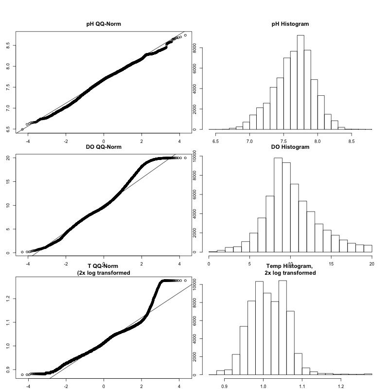
Then I checked out normality. Temperature data was not normal, so I double-log transformed. NOTE: haven’t thrown out any outliers yet; I may after discussing data with Micah. Resulting qqplots & histograms:
Then, I ran the Bartlett Test of Equal Variance for each environmental variable, by each grouping factor.
| Treatment | Habitat | Site | Region | |
|---|---|---|---|---|
| pH-F | 9177.01824 | 518.84135 | 4287.46341 | 3046.27905 |
| pH-P | 0.00000 | 0.00000 | 0.00000 | 0.00000 |
| DO-F | 6629.77718 | 114.20095 | 5479.65027 | 4290.31405 |
| DO-P | 0.00000 | 0.00000 | 0.00000 | 0.00000 |
| T-F | 7745.15337 | 7.18461 | 7666.51686 | 2512.32029 |
| T-P | 0.00000 | 0.00735 | 0.00000 | 0.00000 |
Finally, I ran 1-Way ANOVA tests for each environmental variable, by each grouping factor:
| Treatment | Habitat | Site | Region | |
|---|---|---|---|---|
| pH-F | 5756.8843 | 18550.3358 | 4435.2426 | 5178.1590 |
| pH-P | 0.0000 | 0.0000 | 0.0000 | 0.0000 |
| DO-F | 462.7035 | 172.7403 | 674.5283 | 675.6917 |
| DO-P | 0.0000 | 0.0000 | 0.0000 | 0.0000 |
| T-F | 3327.6405 | 53.9099 | 7441.9589 | 10106.3882 |
| T-P | 0.0000 | 0.0000 | 0.0000 | 0.0000 |
Micah’s suggestions:
- average daily trend plots. Takes hourly averages from midnight to midnight
- 3-5am, and 4-6pm