Measuring QuantSeq larvae
The QuantSeq run I am prepping for will look at gene expression in O. lurida larvae, which were produced by adults that had previously been held in varying winter temperature and pCO2. All larvae were collected and frozen within a day or two of being released from the brood chamber, therefore they should all be at the same developmental stage. The size upon release, however, could be slightly different depending on the larval growth rate, and if larval release is triggered by something (e.g. food, tank cleaning). Since larval size could correspond with developmental stage which impacts gene expression profiles, I measured all the larvae that will also be sequenced.
Methods
While homogenizing frozen larvae with mortar + pestle, I preserved some of the larvae in ethanol, held in a fridge. To measure, I used the Nikon camera + microscope in Jackie’s lab, and the NIS-Element software’s automatic measurement capabilities. Steps:
- Suspend larvae in ethanol with a pipette, transfer to a slide with cover slip
- Capture image of larvae that are lying on their side, so the full width/length could be measured
- Apply a binary layer to the image using the pre-determined threshold setting (based on color). The threshold also uses circularity and size to determine where the binary boundaries occur, and what to include.
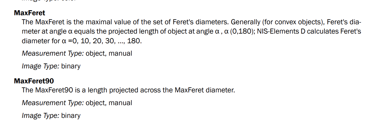
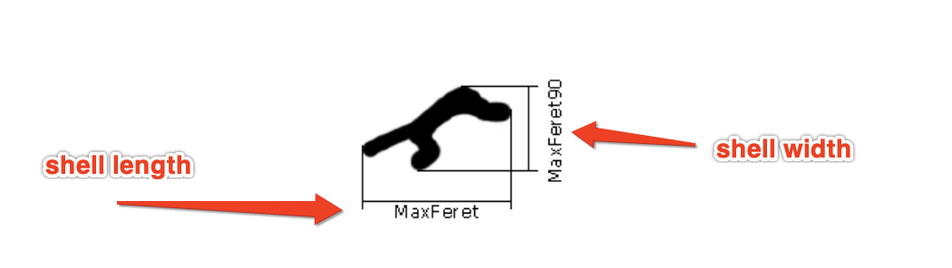
- Use the automatic measurement option to draw perimeters around all binary objects, then generate measurement statistics about each object. Here are details of the measurements I pulled for each object, from the NIS-Element user manual. Note: I believe the MaxFeret is the best representation of shell width, and MaxFeret90 is shell height.


When measuring objects, it’s important to do quality control - some larvae should not be included since they are at a weird angle, or tissue/junk is included in the auto-generated object, thus making the measurements erroneous. After doing this QC, I exported 2 images simultanously: 1) microscope image without any annotations, layers, etc.; 2) binary layer showing objects that were measured, object IDs, and scale bar. It took me a long time to figure out the software, which I don’t think is very intuitive.
Screen recording of measuring larvae:

Results
I measured at minimum 50 larvae from each of my 58 larval sample. Here are some quick and dirty plots of MaxFeret90 (aka shell height) and MaxFeret (aka shell width):
Shell width and height; data from all larvae measured (not standardized across larval pulses):


Shell width & height averages within a larval pulse:


I ran stats on the average shell width ~ treatment:
> larvae.size.mean <- larvae.size %>%
+           group_by(Population, Temperature, pH, Sample) %>%
+           summarise(MaxFeret.mean=mean(MaxFeret), MaxFeret90.mean=mean(MaxFeret90), date=mean(DateCollected))
> hist(larvae.size.mean$MaxFeret.mean)
> shapiro.test(larvae.size.mean$MaxFeret.mean)

  Shapiro-Wilk normality test

data:  larvae.size.mean$MaxFeret.mean
W = 0.98548, p-value = 0.6162

> bartlett.test(MaxFeret.mean ~ pH, data=larvae.size.mean)

  Bartlett test of homogeneity of variances

data:  MaxFeret.mean by pH
Bartlett's K-squared = 1.9194, df = 1, p-value = 0.1659

> bartlett.test(MaxFeret.mean ~ Temperature, data=larvae.size.mean)

  Bartlett test of homogeneity of variances

data:  MaxFeret.mean by Temperature
Bartlett's K-squared = 1.203, df = 1, p-value = 0.2727

> summary(aov(MaxFeret.mean ~ Temperature*pH, data=larvae.size.mean))
               Df Sum Sq Mean Sq F value Pr(>F)
Temperature     1   86.9   86.88   5.784 0.0191 *
pH              1   67.9   67.86   4.518 0.0374 *
Temperature:pH  1   10.8   10.82   0.721 0.3991
Residuals      64  961.3   15.02
---
Signif. codes:  0 ‘***’ 0.001 ‘**’ 0.01 ‘*’ 0.05 ‘.’ 0.1 ‘ ’ 1
> TukeyHSD(aov(MaxFeret.mean ~ Temperature*pH, data=larvae.size.mean))
  Tukey multiple comparisons of means
    95% family-wise confidence level

Fit: aov(formula = MaxFeret.mean ~ Temperature * pH, data = larvae.size.mean)

$Temperature
         diff       lwr      upr     p adj
10-6 2.264579 0.3835259 4.145632 0.0190728

$pH
                diff        lwr      upr     p adj
low-ambient 1.844838 -0.0337701 3.723447 0.0541359

$`Temperature:pH`
                           diff        lwr      upr     p adj
10:ambient-6:ambient  2.1486852 -1.8472133 6.144584 0.4926858
6:low-6:ambient       1.2038439 -2.8156759 5.223364 0.8587164
10:low-6:ambient      5.0921551  0.5841736 9.600137 0.0207176
6:low-10:ambient     -0.9448413 -3.9279133 2.038231 0.8373728
10:low-10:ambient     2.9434699 -0.6709563 6.557896 0.1491559
10:low-6:low          3.8883112  0.2477877 7.528835 0.0318319
Next steps
However, it’s important to consider that the # larval pulses included in these data are unbalanced:
| Population | Temperature | pH | # larval groups |
|---|---|---|---|
| Dabob Bay | 6 | ambient | 1 |
| Dabob Bay | 6 | low | 3 |
| Dabob Bay | 10 | ambient | 4 |
| Dabob Bay | 10 | low | 4 |
| Fidalgo Bay | 6 | ambient | 2 |
| Fidalgo Bay | 6 | low | 7 |
| Fidalgo Bay | 10 | ambient | 5 |
| Fidalgo Bay | 10 | low | 3 |
| Oyster Bay C1 | 6 | ambient | 2 |
| Oyster Bay C1 | 6 | low | 8 |
| Oyster Bay C1 | 10 | ambient | 12 |
| Oyster Bay C1 | 10 | low | 2 |
| Oyster Bay C2 | 6 | ambient | 4 |
| Oyster Bay C2 | 6 | low | 5 |
| Oyster Bay C2 | 10 | ambient | 3 |
| Oyster Bay C2 | 10 | low | 3 |
I need to measure the following larvae - missed these since I already had RNA:
| Date Collected | Spawning Group | Population | Treatment | Larval sample # | RNA Sample # | Date homogenized |
|---|---|---|---|---|---|---|
| 5/23/17 | SN-10 Low B | Oyster Bay C1 | 10 Low | 08-A | 43 | na |
| 5/26/17 | SN-10 Low B | Oyster Bay C1 | 10 Low | 24-A | 46 | na |
| 5/27/17 | SN-10 Low B | Oyster Bay C1 | 10 Low | 26-A | 47 | na |
| 5/31/17 | SN-10 Low A | Oyster Bay C1 | 10 Low | 32-A | 44 | na |
| 6/24/17 | SN-10 Low A | Oyster Bay C1 | 10 Low | 79-A | 45 | na |
| 5/23/17 | SN-6 Ambient B | Oyster Bay C1 | 6 Ambient | 10-A | 35 | na |
| 6/6/17 | SN-6 Ambient B | Oyster Bay C1 | 6 Ambient | 48-A | 39 | na |
| 6/15/17 | SN-6 Ambient B | Oyster Bay C1 | 6 Ambient | 69-A | 37 | na |
| 6/19/17 | SN-6 Ambient A | Oyster Bay C1 | 6 Ambient | 77-A | 34 | na |