Post Skyline Data Processing

Please see my Geoduck-DNR Repo, June Analyses folder for most up-to-date version of this process.

In this workflow I process Skyline data to assess proteins expressed in Geoduck during outplant in 5 sites throughout Puget Sound in 2 treatments: eelgrass, and bare (no eelgrass).

Pertinent files for ths process: R code, Biostats.R

Step 1: Export report from Skyline

screen shots TBD

Step 2: Add site/treatment to columns, remove #N/A, and normalize based on Total Ion Current

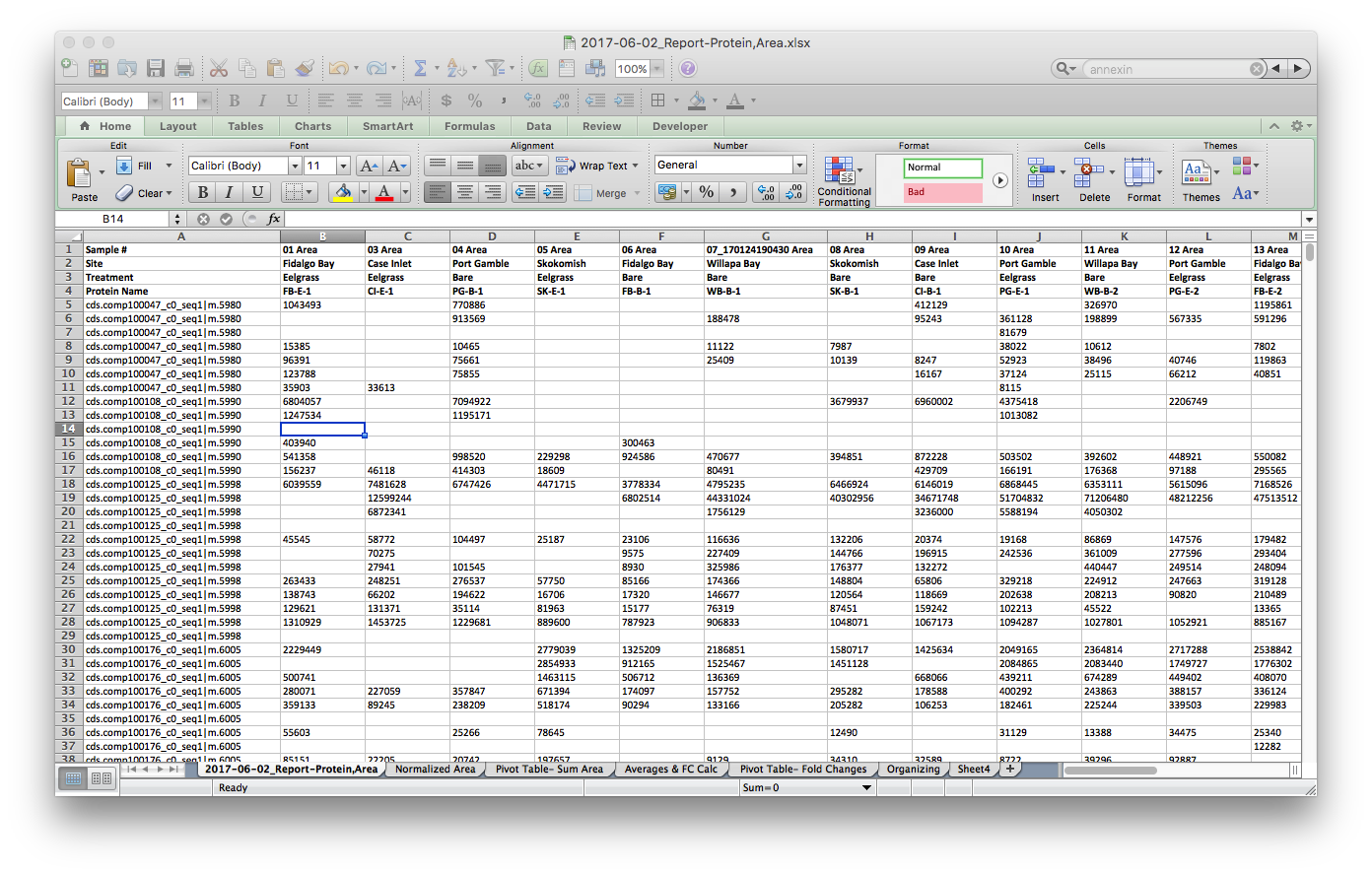
The raw file from Skyline, opened in Excel, looks like this:

I used Excel to make these small modifications. Yes, I could have dones this in R, but I didn’t (next time I will). I referenced my Mass Spec Sequence File to match file names to sample numbers, and then my Geoduck Organization file to match sample names to site and treatment. To edit all #N/A I used the Find & Replace tool. Skyline data ID'd and #N/A removed

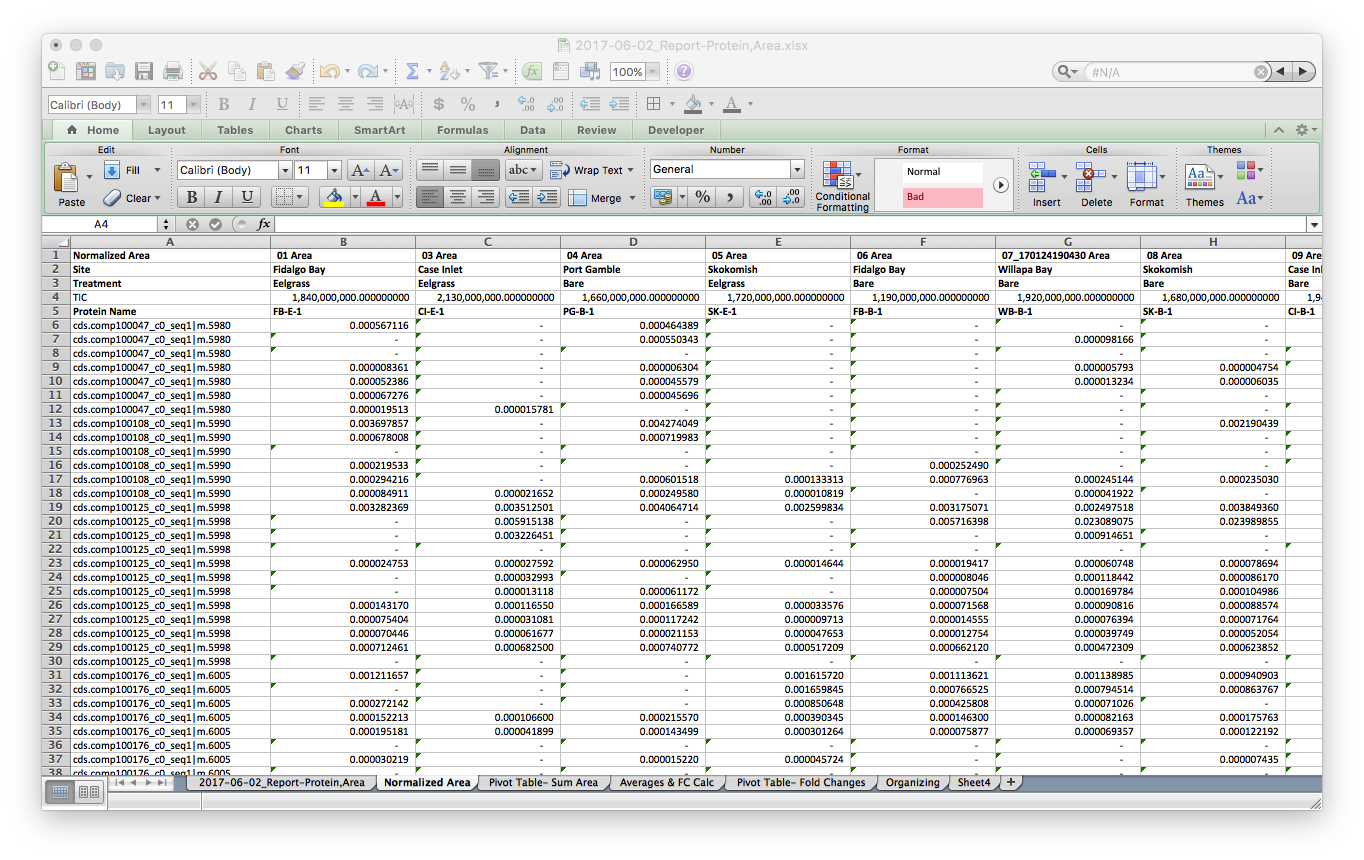
Finally, I opened a new tab and normalized the data by the Total Ion Current (TIC) for each sample. TIC data was given to me from Emma. Skyline data normalized by TIC

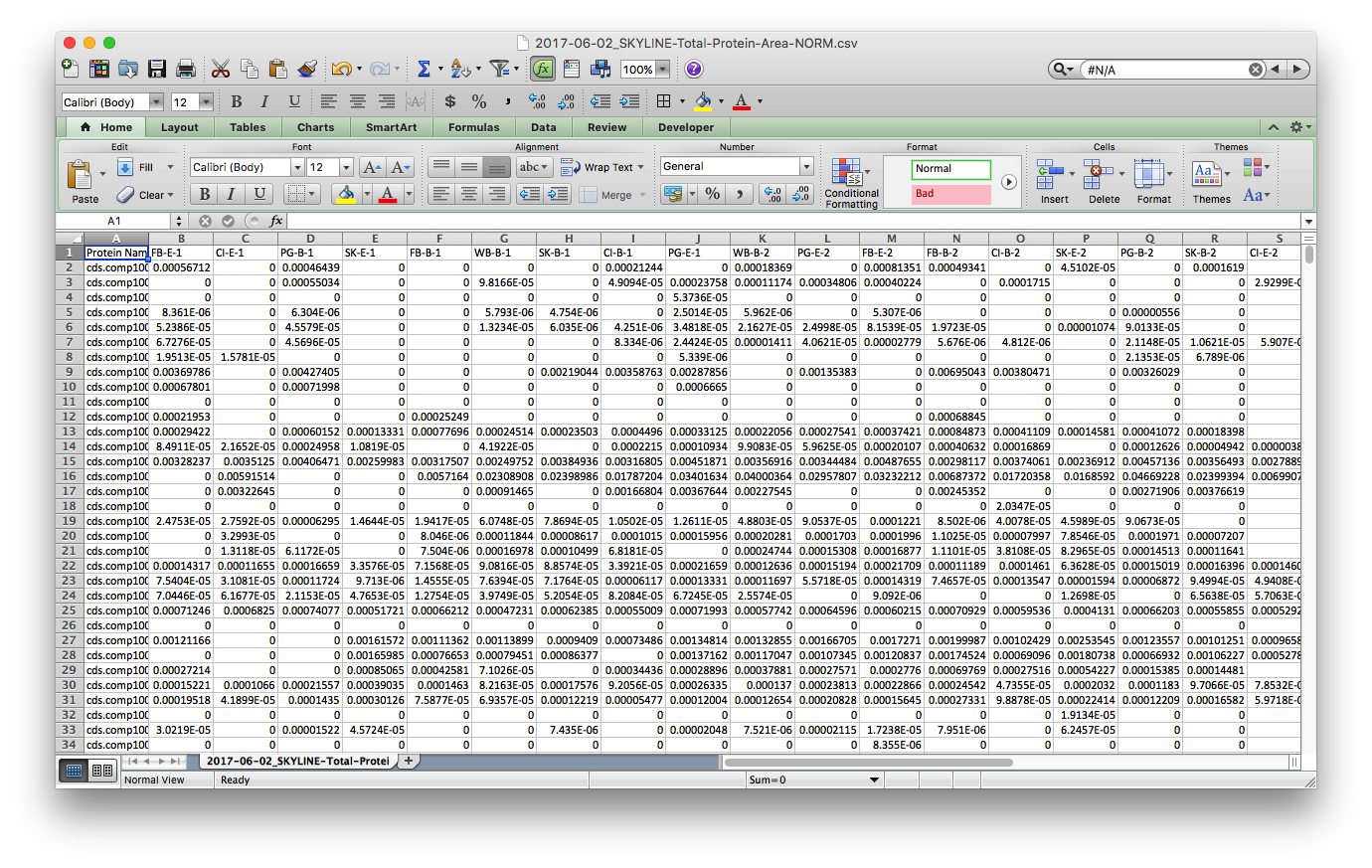
I saved this tab as a new file, 2017-06-02_SKYLINE-Total-Protein-Area-NORM.csv2017-06-02_SKYLINE-Total-Protein-Area-NORM.csv, cleaned up the header with simplified sample codes: e.g. FB-E-1 & CI-B-2 for Fidalgo Bay Eelgrass technical rep 1, Case Inlet Bare technical replicate 2, respectively. Also notice that all the n/a spaces are showing up as 0. I’ll take care of this in R

Normalized Skyline Data for R

Step 3: Read data into R and play with it. I borrowed a lot of this script from Yaamini, with some modifications - thanks Yaamini!

### Import Dataset ### 
### Note: this dataset has already been massaged in Excel: sum area by protein, normalized by TIC, all n/a's removed (replaced with zeros), and columns renamed
setwd("~/Documents/Roberts Lab/Geoduck-DNR/Analyses/2017-June_Analyses")
NormProtArea <- read.csv("2017-06-02_SKYLINE-Total-Protein-Area-NORM.csv", header=TRUE, na.strings = "0") # import local file
head(NormProtArea)

imported data

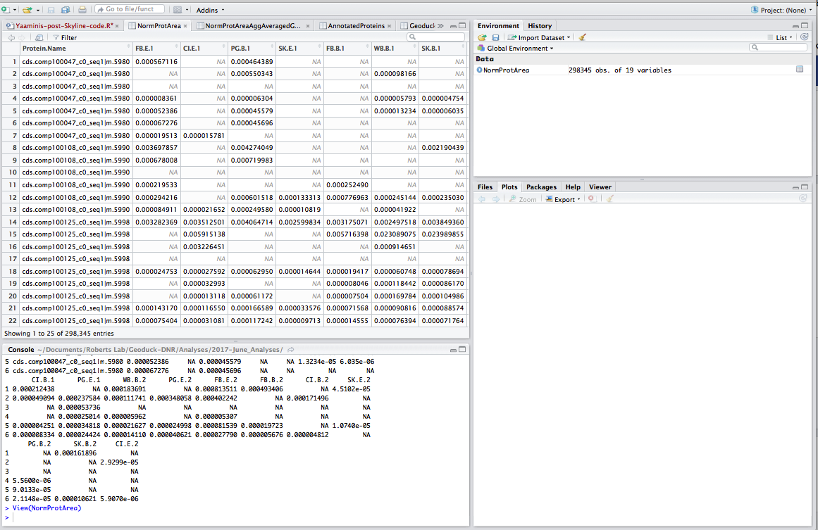
Step 4: Aggregate transition area by protein. Data currently represents the area under the curve for each transition. To find the total area per protein I use the `aggregate()` function to sum all transition areas by protein.

### SUM TRANSITION AREA BY PROTEIN ### 
# The "Area" values (which have already been normalized by TIC) are peak area for each transition. Sum them to determine total area for each protein

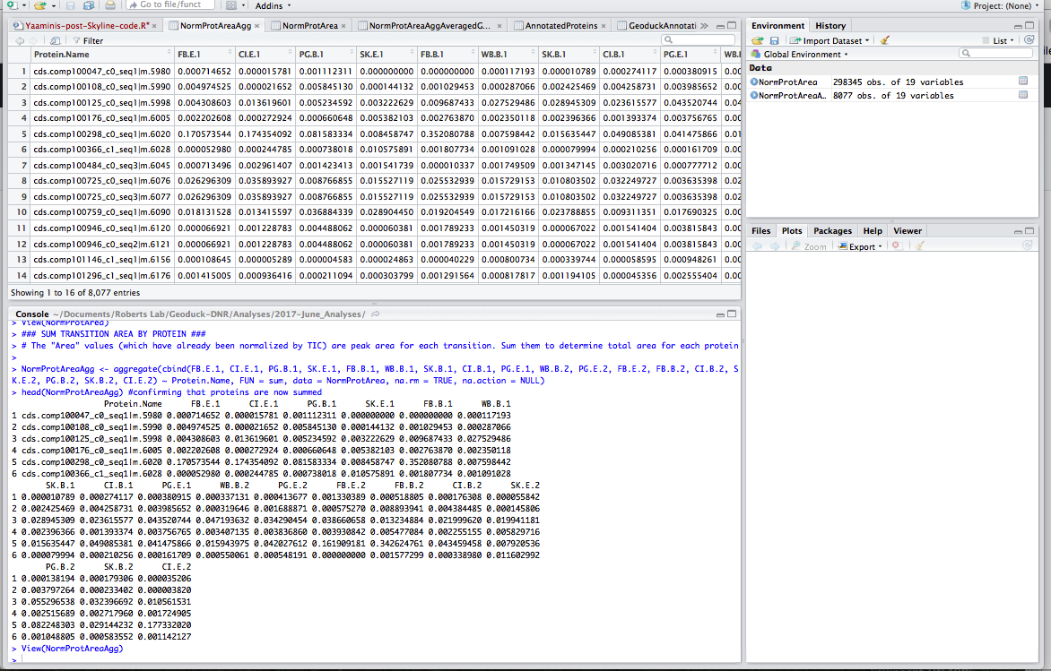
NormProtAreaAgg <- aggregate(cbind(FB.E.1, CI.E.1, PG.B.1, SK.E.1, FB.B.1, WB.B.1, SK.B.1, CI.B.1, PG.E.1, WB.B.2, PG.E.2, FB.E.2, FB.B.2, CI.B.2, SK.E.2, PG.B.2, SK.B.2, CI.E.2) ~ Protein.Name, FUN = sum, data = NormProtArea, na.rm = TRUE, na.action = NULL)
head(NormProtAreaAgg) #confirming that proteins are now summed

agg data

Step 5: Average technical replicates. Each sample ran through the MS/MS twice; here I calculate the average for each treatment/site combo:

#### AVERAGE REPLICATES #### 
# FYI No eelgrass sample for Willapa Bay

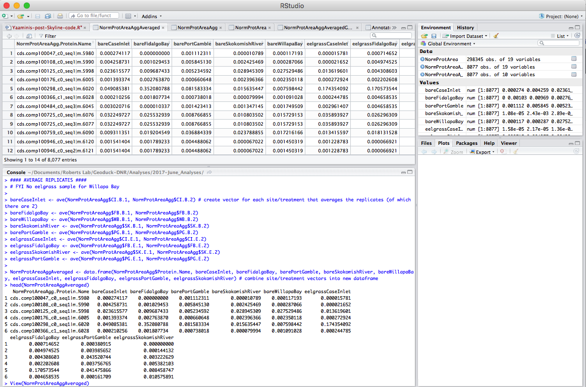
bareCaseInlet <- ave(NormProtAreaAgg$CI.B.1, NormProtAreaAgg$CI.B.2) # create vector for each site/treatment that averages the replicates (of which there are 2)
bareFidalgoBay <- ave(NormProtAreaAgg$FB.B.1, NormProtAreaAgg$FB.B.2)
bareWillapaBay <- ave(NormProtAreaAgg$WB.B.1, NormProtAreaAgg$WB.B.2)
bareSkokomishRiver <- ave(NormProtAreaAgg$SK.B.1, NormProtAreaAgg$SK.B.2)
barePortGamble <- ave(NormProtAreaAgg$PG.B.1, NormProtAreaAgg$PG.B.2)
eelgrassCaseInlet <- ave(NormProtAreaAgg$CI.E.1, NormProtAreaAgg$CI.E.2)
eelgrassFidalgoBay <- ave(NormProtAreaAgg$FB.E.1, NormProtAreaAgg$FB.E.2)
eelgrassSkokomishRiver <- ave(NormProtAreaAgg$SK.E.1, NormProtAreaAgg$SK.E.2)
eelgrassPortGamble <- ave(NormProtAreaAgg$PG.E.1, NormProtAreaAgg$PG.E.2)

NormProtAreaAggAveraged <- data.frame(NormProtAreaAgg$Protein.Name, bareCaseInlet, bareFidalgoBay, barePortGamble, bareSkokomishRiver,    bareWillapaBay, eelgrassCaseInlet, eelgrassFidalgoBay, eelgrassPortGamble, eelgrassSkokomishRiver) # combine site/treatment vectors into    new dataframe
head(NormProtAreaAggAveraged)

ave data

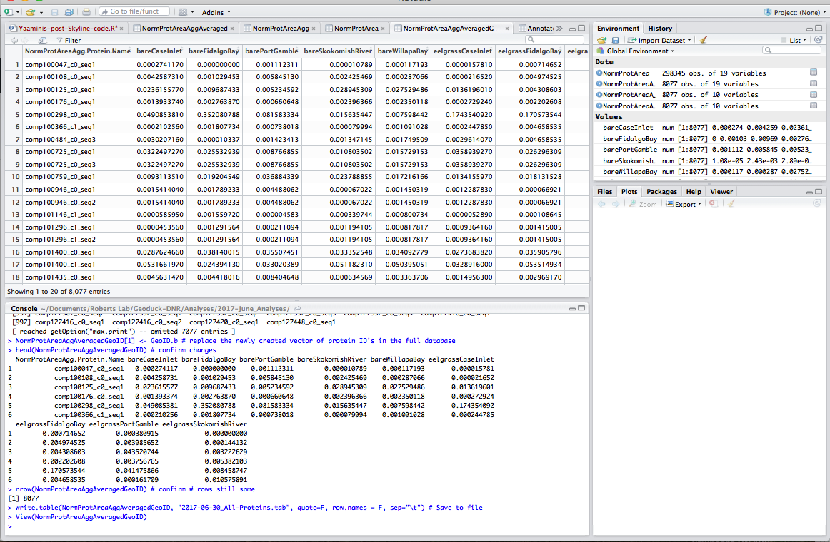
Step 6: Prep file to merge with annotations. The Protein ID in my Skyline files are formatted differently from the GeoID in my annotation file. Here I edit out the extra string (in bold), cds.comp100047_c0_seq1|m.5980

### EDITING GEOID NAME TO MATCH ANNOTATED FILE ### 
NormProtAreaAggAveragedGeoID <- NormProtAreaAggAveraged # copy database, create new one to be used to join to annotated file
GeoID.a <- (gsub("cds.", "", NormProtAreaAggAveragedGeoID$NormProtAreaAgg.Protein.Name, fixed=TRUE)) # remove cds. from protein ID
GeoID.b <- (gsub("\\|m.*", "", GeoID.a)) # remove |m.#### from protein ID
noquote(GeoID.b) # remove quotes from resulting protein ID
NormProtAreaAggAveragedGeoID[1] <- GeoID.b # replace the newly created vector of protein ID's in the full database
head(NormProtAreaAggAveragedGeoID) # confirm changes
nrow(NormProtAreaAggAveragedGeoID) # confirm # rows still same
write.table(NormProtAreaAggAveragedGeoID, "2017-06-30_All-Proteins.tab", quote=F, row.names = F, sep="\t") # Save to file

edit id

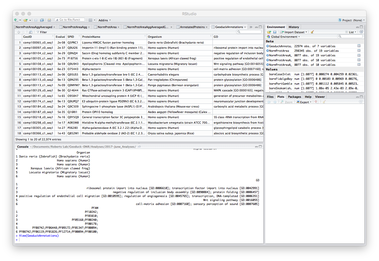
Step 7: Upload annotations. This file is the annotated proteins found via geoduck gonad transcriptome.

### UPLOAD ANNOTATED GEODUCK PROTEOME FROM URL ###
GeoduckAnnotations <- read.table(
    "https://raw.githubusercontent.com/sr320/paper-pano-go/master/data-results/Geo-v3-join-uniprot-all0916-condensed.tab",
    sep="\t", header=TRUE, fill=TRUE, stringsAsFactors = FALSE, quote="") #fill=TRUE for empty spaces 
nrow(GeoduckAnnotations) # check that the # rows matches the source (I know this from uploading to Galaxy; not sure how else to do it)
ncol(GeoduckAnnotations) # check that the # columns matches the source
head(GeoduckAnnotations) # inspect; although it's easier to "view" in RStudio

geo annotations file

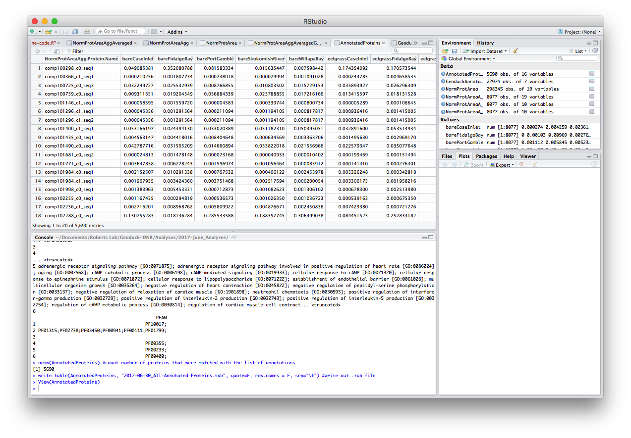
Step 8: Merge the 8076 total proteins found in my samples with the annotations. After merge, there are 5,690 annotated proteins in my data. Annotated file is 2017-06-30_All-Annotated-Proteins.tab

# MERGE ANNOTATIONS WITH ALL MY PROTEINS ### 
AnnotatedProteins <- merge(x = NormProtAreaAggAveragedGeoID, y = GeoduckAnnotations, by.x="NormProtAreaAgg.Protein.Name", by.y="GeoID")
head(AnnotatedProteins) #confirm merge
nrow(AnnotatedProteins) #count number of proteins that were matched with the list of annotations
write.table(AnnotatedProteins, "2017-06-30_All-Annotated-Proteins.tab", quote=F, row.names = F, sep="\t") #write out .tab file

merged annotation

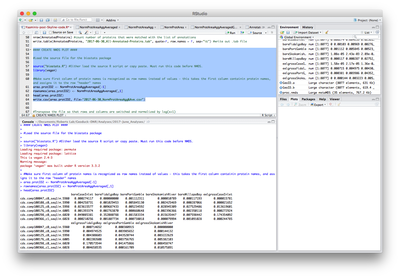
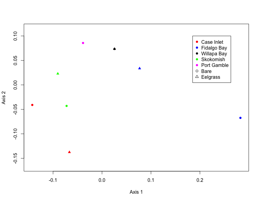
Step 9: Make NMDS plot to assess overall site relatedness. Again, thanks to Yaamini for providing me the code! Note: I saved the biostats.R code as an R script in my repo/working directory

    #### CREATE NMDS PLOT ####

    #Load the source file for the biostats package

    source("biostats.R") #Either load the source R script or copy paste. Must run this code before NMDS.
    library(vegan)

    #Make sure first column of protein names is recognized as row names instead of values - this takes the first column containin protein names, and assigns it to the row "header" names 
    area.protID <- NormProtAreaAggAveraged[-1]
    rownames(area.protID) <- NormProtAreaAggAveraged[,1]
    head(area.protID)
    write.csv(area.protID, file="2017-07-04_NormProtAreaAgg&Ave.csv") #write this file out for safe keeping 

nmds

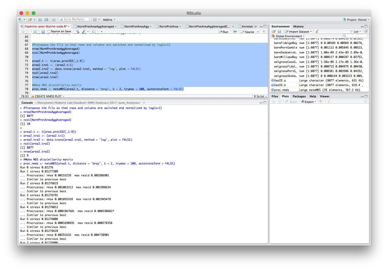
    #Transpose the file so that rows and columns are switched 
    area.protID.t <- t(area.protID[,1:9])
    nrow(NormProtAreaAggAveraged) # Compare row and column lengths before and after transposing
    ncol(NormProtAreaAggAveraged) 
    nrow(area.protID.t)
    ncol(area.protID.t)

    #Make MDS dissimilarity matrix
    proc.nmds <- metaMDS(area.protID.t, distance = 'bray', k = 2, trymax = 100, autotransform = FALSE)

draw nmds box

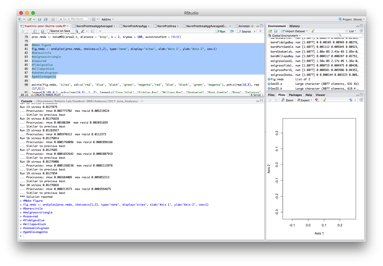
    #Make figure
    fig.nmds <- ordiplot(proc.nmds, choices=c(1,2), type='none', display='sites', xlab='Axis 1', ylab='Axis 2', cex=1)
    #bare=circle
    #eelgrass=triangle
    #case=red
    #fidalgo=blue
    #willapa=black
    #skokomish=green
    #gamble=magenta

draw nmds box

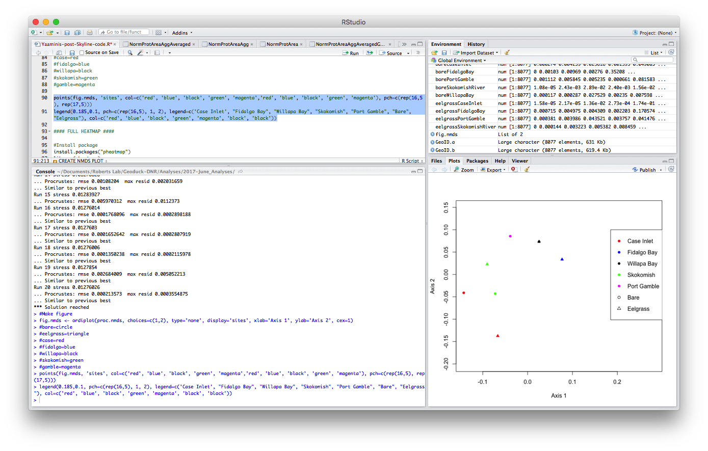
    points(fig.nmds, 'sites', col=c('red', 'blue', 'black', 'green', 'magenta','red', 'blue', 'black', 'green', 'magenta'), pch=c(rep(16,5), rep(17,5)))
    legend(0.185,0.1, pch=c(rep(16,5), 1, 2), legend=c('Case Inlet', "Fidalgo Bay", "Willapa Bay", "Skokomish", "Port Gamble", "Bare", "Eelgrass"), col=c('red', 'blue', 'black', 'green', 'magenta', 'black', 'black'))

apply points NMDS plot

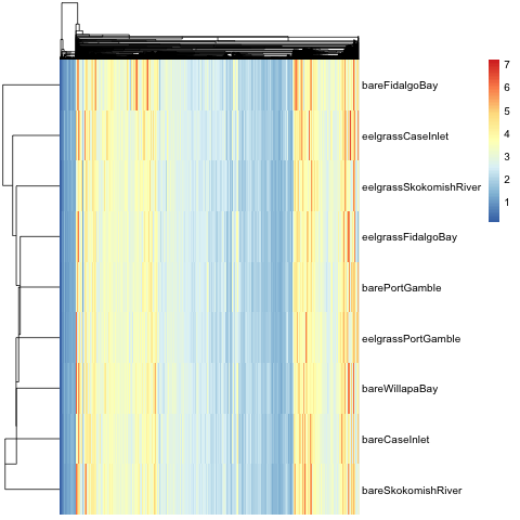
FULL HEATMAP

    #Install package
    install.packages("pheatmap")
    library(pheatmap)

    #Data should be log(x) or log(x+1) transformed for this analysis. I thus invert my data (since I had normalized by TIC so values were <1), then log transform.

    #Invert data then log transformation for heat map
    area.protID.t.inv <- (1/area.protID.t)
    is.na(area.protID.t.inv) <- sapply(area.protID.t.inv, is.infinite) # change "Inf" to "NA"
    area.protID.t.inv.log <- data.trans(area.protID.t.inv, method = 'log', plot = FALSE)
    ncol(area.protID.t.inv.log)
    nrow(area.protID.t.inv.log)

    #Create heatmap
    pheatmap(area.protID.t.inv.log, cluster_rows = T, cluster_cols = T, clustering_distance_rows = 'euclidean', clustering_distance_cols = 'euclidean', clustering_method = 'median', show_rownames = T, show_colnames = F)

heatmap

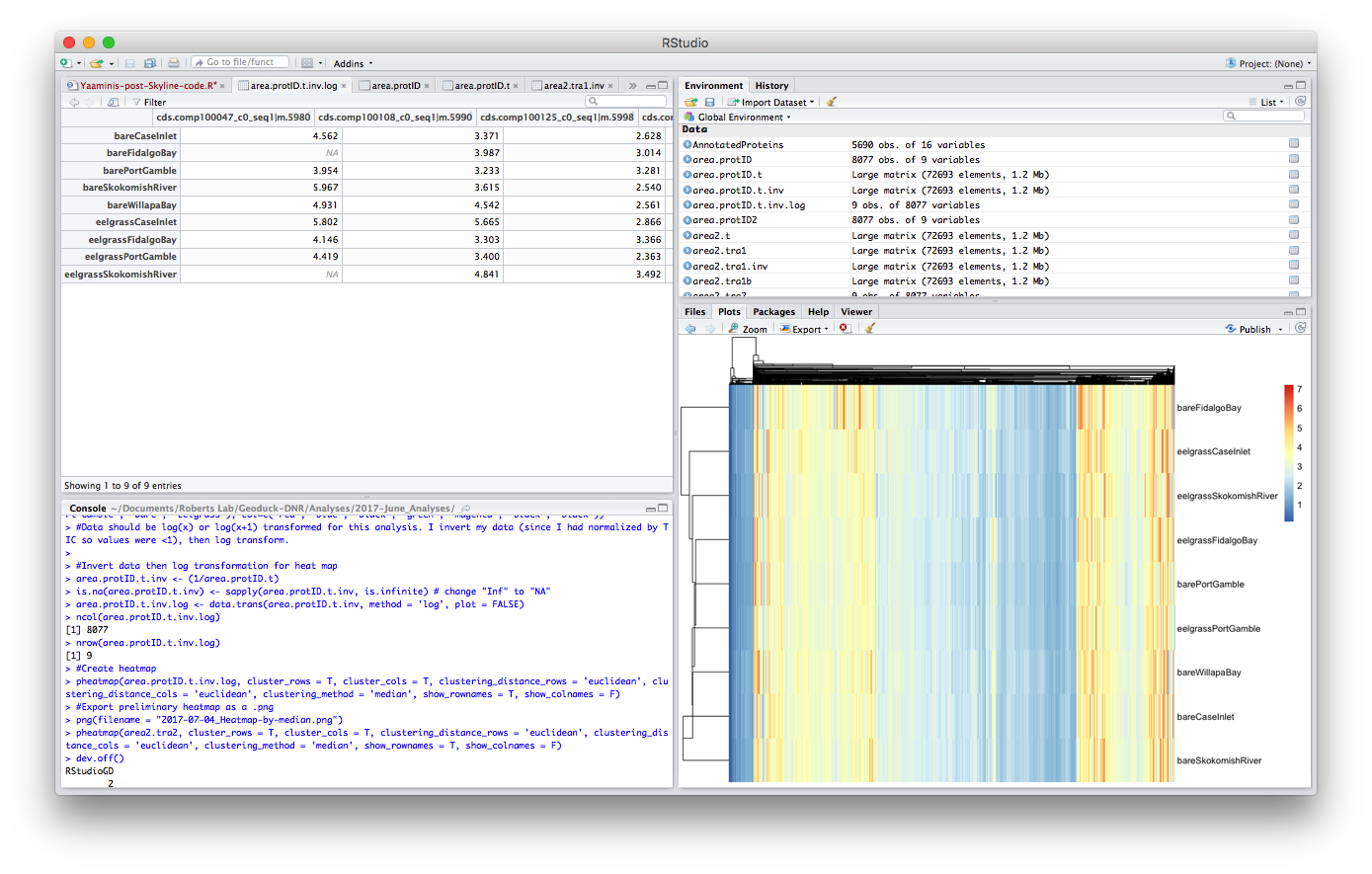
    #Export preliminary heatmap as a .png
    png(filename = "2017-07-04_Heatmap-by-median.png")
    pheatmap(area2.tra2, cluster_rows = T, cluster_cols = T, clustering_distance_rows = 'euclidean', clustering_distance_cols = 'euclidean', clustering_method = 'median', show_rownames = T, show_colnames = F)
    dev.off()

heatmap image

Step 11: Calculate coefficients of variances & means, and plot. I did this to visualize how variable the proteins are- plot TBD

    ### Find COEFFICIENT OF VARIANCES & MEANS ###

    ProtVariance <- c(var(area2.tra2[-1], area2.tra2[1], na.rm=TRUE))
    ProtMeans <- c(colMeans(area2.tra2[-1], na.rm=TRUE))
    ProtVar.Means <- data.frame(,y)
    ProtVar.Means <- data.frame(NormProtAreaAggAveraged[1], ProtMeans, ProtVariance)
    
    nrow(NormProtAreaAggAveraged[1])
    length(ProtMeans)
    length(ProtVariance)
    head(ProtMeans)
    ncol(ProtMeans)

Written on July 4, 2017