Taking a simpler approach to identifying correlations between environmental data and protein abundances. Goals of today was to:

1. Subselect salinity data, generate summary stats, to be able to include in analysis
2. Generate correlation plots with R^2 and P-values between differentially abundant proteins and environmental summary stats
3. From plots, select env. summary stats to use in 1) multiple linear regression model & 2) structural equation model
4. Generate correlation plots with selected env. variables to identify potential interactions
5. Run multiple linear regression model
6. Interpret results
7. Revise paper to include results from these tasks

1. Subselected salinity data, generate summary stats, include in analysis

The environmental data manipulation referenced in this post was executed in the Stats 2 R script.

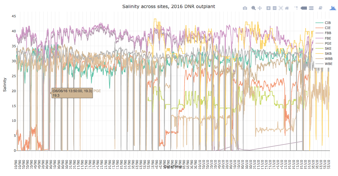
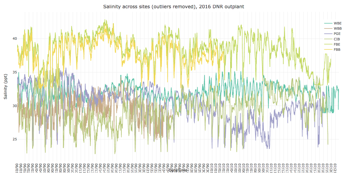
In one of our team meetings we made the determination to ignore salinity data for the time being, since several probes malfunctioned. Up until this point I have performed all tasks/stats on salinity data alongside the other parameters, but ignored salinity when analyzing correlations. Today I generated correlation plots and found salinity may play a role. So, I decided to clean up salinity data as much as I could to include in my analysis. To do so, I reviewed raw salinity data via this plotly plot. Determined that the following salinity data needed to be removed due to probe malfunction: All CIE; FBB > 7/3 @ 09:50; WBB > 6/25 @ 05:30. I then removed all outliers from the updated salinity time-series data, and re-plotted. This is the resulting plot

Raw salinity data:

Bad data & outliers removed:

2. Generated correlation plots with R^2 and P-values between differentially abundant proteins and environmental summary stats

The rest of this post refers to actions taken in the Stats 4 R script.

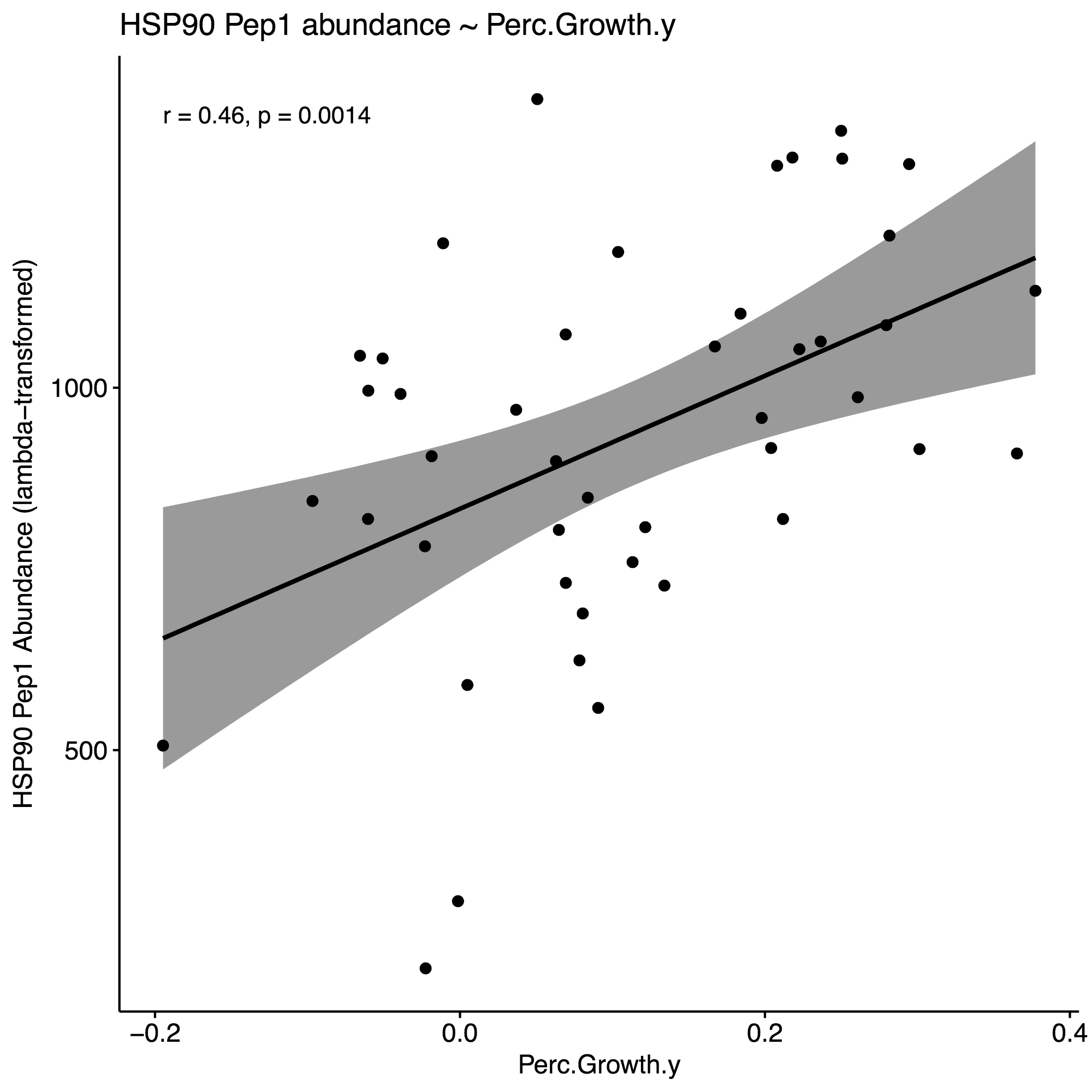
Discovered the excellent ggscatter function in the ggpubr library to generate correlation plots. I generated correlation plots for the 3 differentially abundant proteins (HSP90, Puromycin-sensitive aminopeptidase, Trifunctional Enzyme). At first I was going to just use Pep1 (the most abundant peptide from each protein) to generate these plots. Instead, I z-transformed all peptide abundance data so they were all on the same scale, and thus could regress all peptides from each protein against environmental paramters.
It’s a good idea to quickly summarize how I’ve manipulated peptide abundance data in this project:

1. lambda-transformed abundance by each protein to create normal distributions, then compared across habitats, sites, and regions using ANOVA
2. z-transformed by each peptide ((X-mean)/SD), then ran correlation analysis against each environmental parameter

• Heat Shock Protein 90 correlation plots
• Puromycin-sensitive aminopeptidase
• Trifuctional-enzyme

3. From plots, selected env. summary stats to use in models

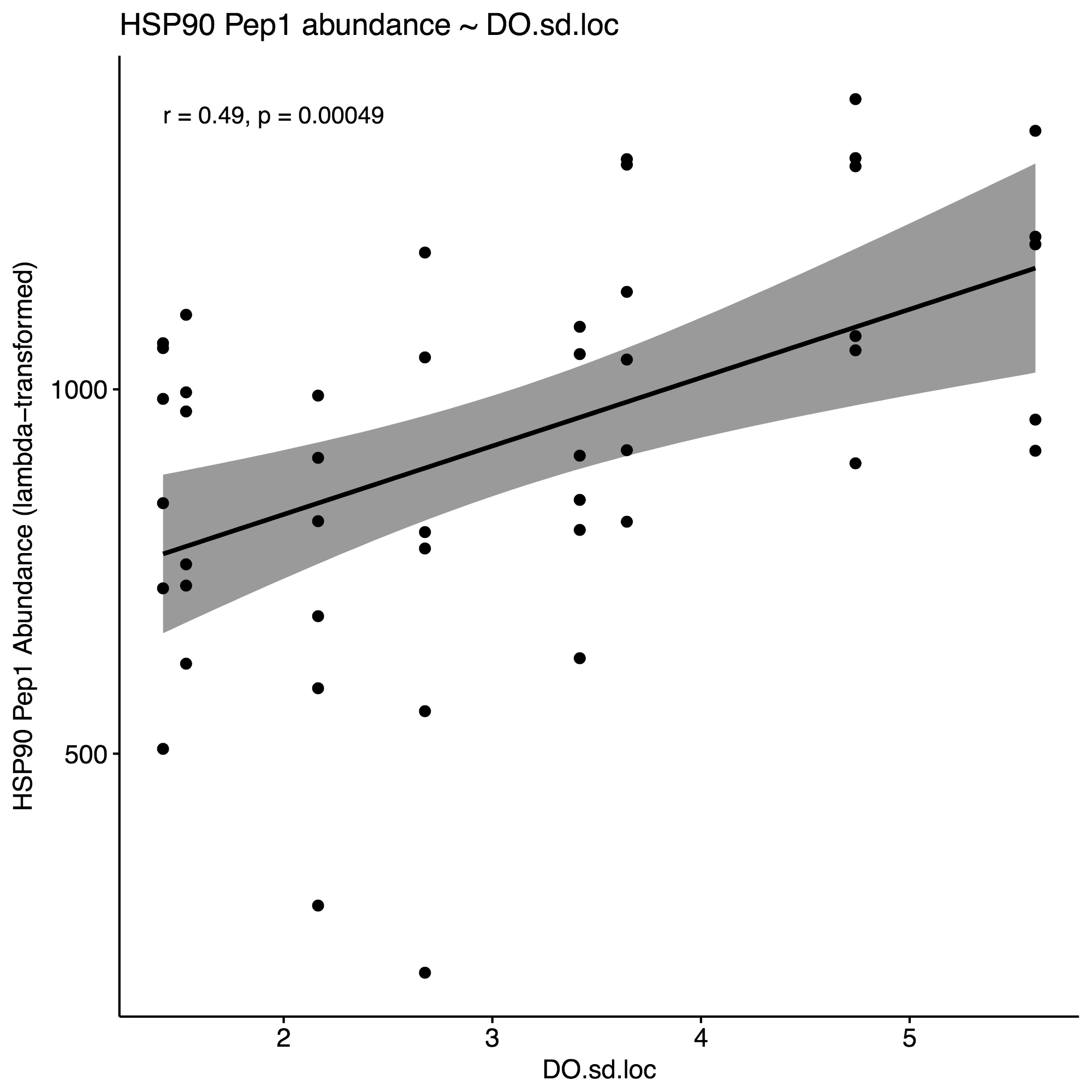
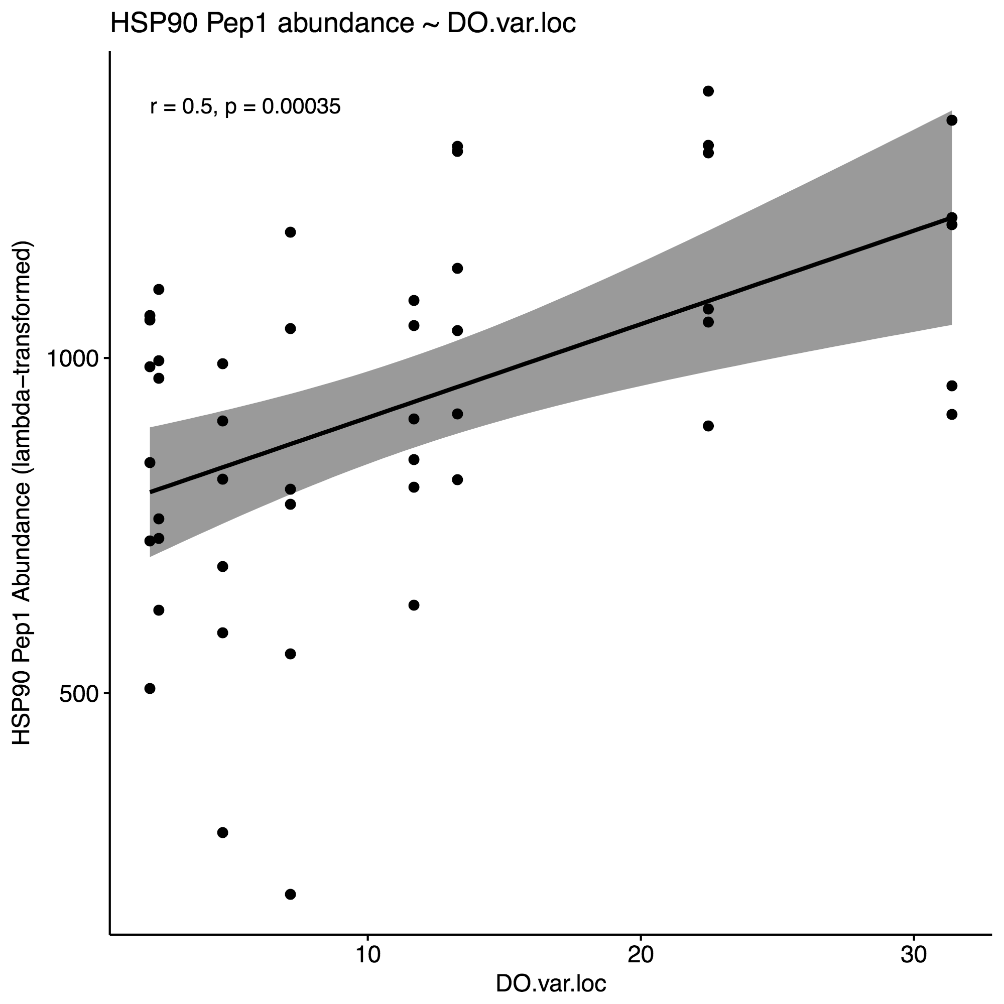
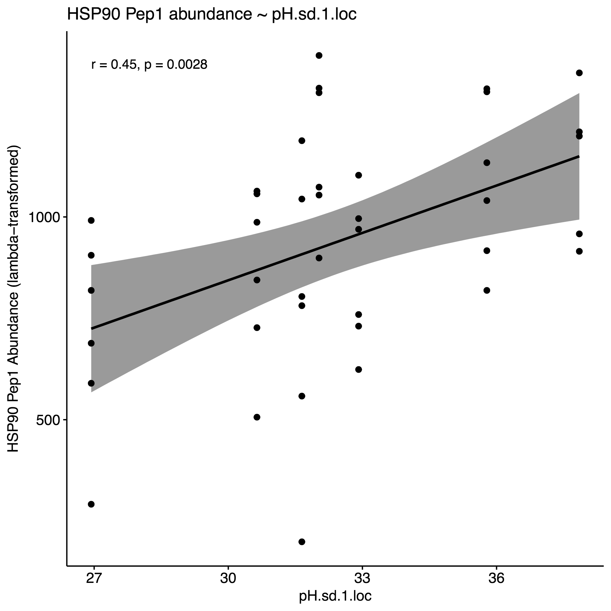
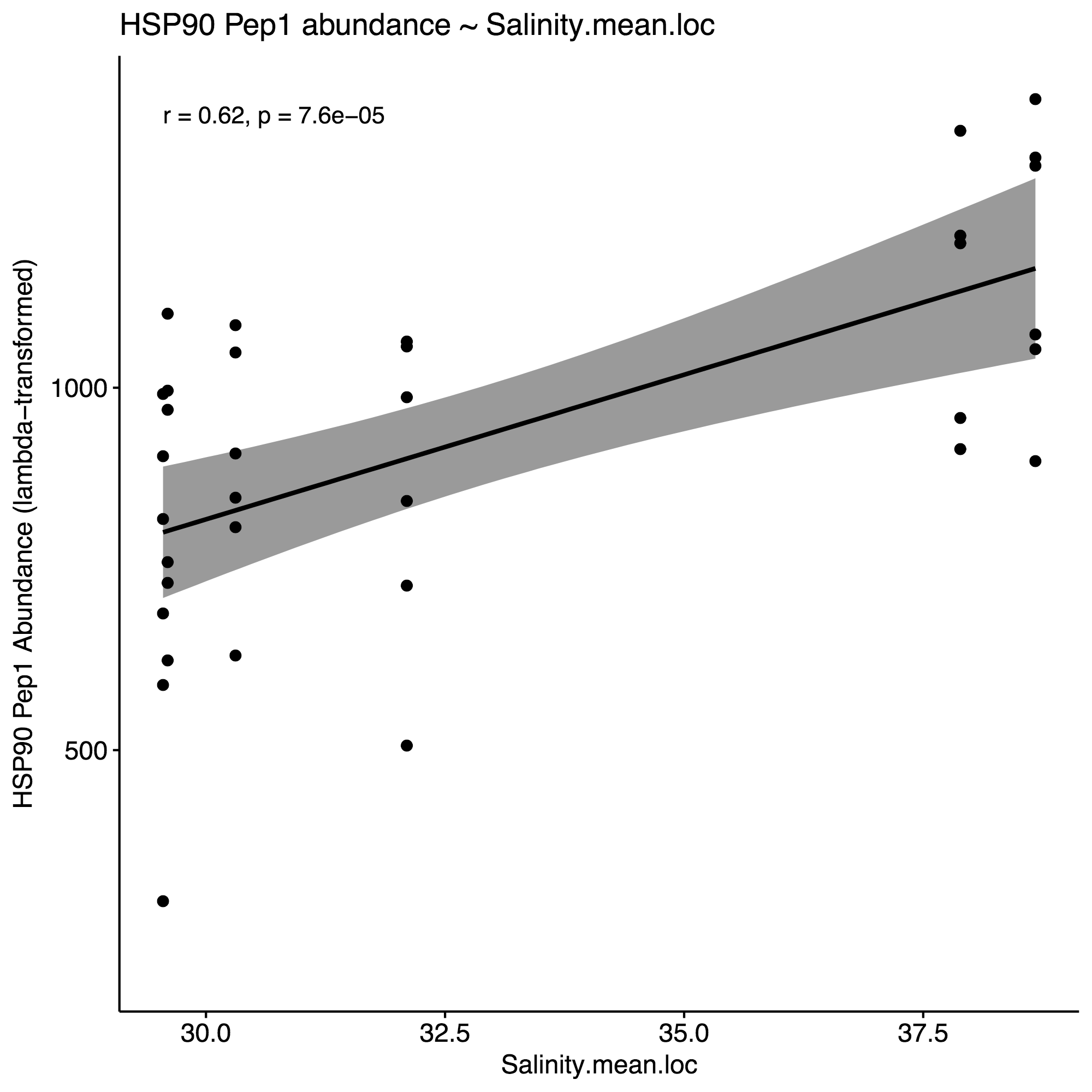
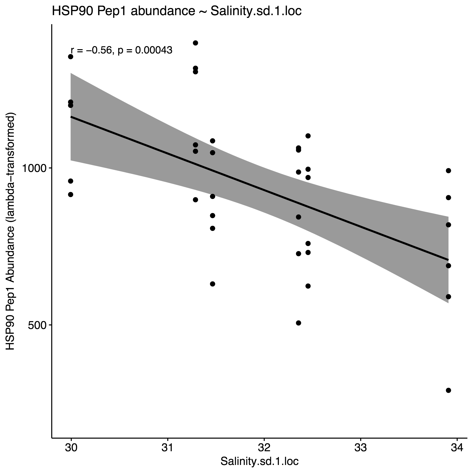
Selected the following environmental parameters per the respective proteins for model constructions, using an approximate alpha=0.01 as cutoff: % Growth, DO.sd, DO.var, pH.sd.1, salinity.mean, salinity.sd.1. Here are the correlation plots for these parameters, using HSP90 for the purposes of this example:

4. Generate correlation plots with selected env. variables to identify potential interactions

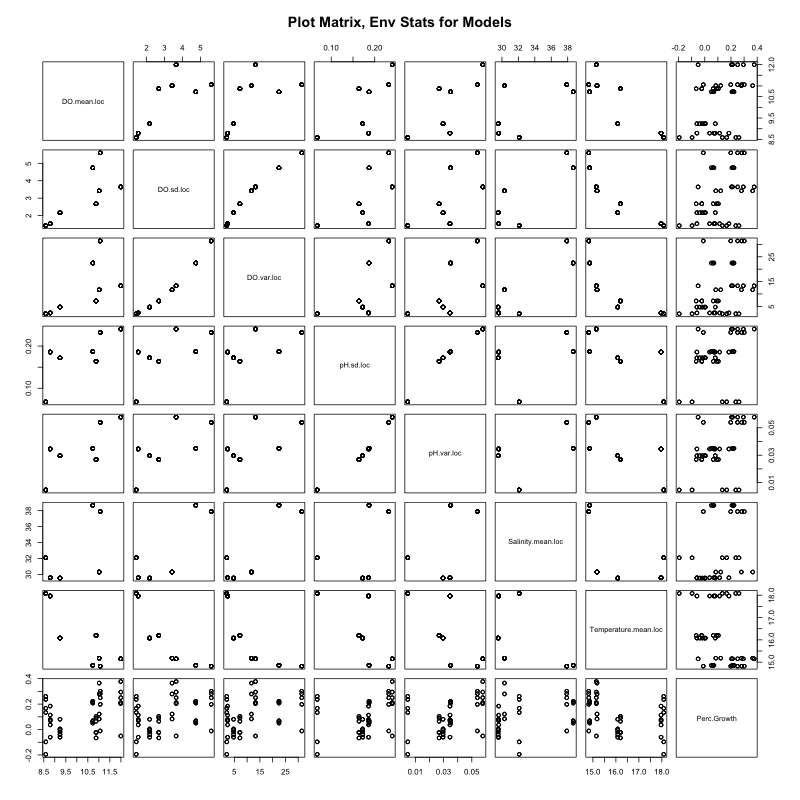
Generated a correlation plot with the pairs() function to identify any environmental parameters that are highly correlated; if identified, I can leave one of the two correlated metrics out of my linear model. From the correlation plot, it appears that:

• DO.sd & DO.var highly correlated. Select DO.sd since it’s correlation p=value is slightly smaller
• pH.sd & pH.var highly correlated. Select pH.var since it’s correlation p=value is smaller and r value higher

5. Run multiple linear regression model

Ran the following model and viewed summary:

Call:
lm(formula = value ~ DO.mean.loc.Z + DO.sd.loc.Z + pH.var.loc.Z + 
    Salinity.mean.loc.Z + Temperature.mean.loc.Z, data = data.pepsum.Env.Stats.HSP90.Z, 
    singular.ok = TRUE)

Residuals:
    Min      1Q  Median      3Q     Max 
-1.7794 -0.4787  0.1177  0.5790  1.2928 

Coefficients: (1 not defined because of singularities)
                       Estimate Std. Error t value Pr(>|t|)   
(Intercept)              0.2450     0.5825   0.421  0.67510   
DO.mean.loc.Z            0.6813     1.1876   0.574  0.56776   
DO.sd.loc.Z             -1.0086     0.9314  -1.083  0.28206   
pH.var.loc.Z             0.3494     0.2268   1.541  0.12723   
Salinity.mean.loc.Z      1.0207     0.3477   2.935  0.00432 **
Temperature.mean.loc.Z       NA         NA      NA       NA   
---
Signif. codes:  0 ‘***’ 0.001 ‘**’ 0.01 ‘*’ 0.05 ‘.’ 0.1 ‘ ’ 1

Residual standard error: 0.7499 on 82 degrees of freedom
  (54 observations deleted due to missingness)
Multiple R-squared:  0.4062,	Adjusted R-squared:  0.3772 
F-statistic: 14.02 on 4 and 82 DF,  p-value: 9.27e-09

Also ran anova() on the model:

> anova(lm.HSP90)
Analysis of Variance Table

Response: value
                    Df Sum Sq Mean Sq F value   Pr(>F)    
DO.mean.loc.Z        1 25.041 25.0415 44.5306 2.74e-09 ***
DO.sd.loc.Z          1  0.575  0.5754  1.0232 0.314744    
pH.var.loc.Z         1  1.077  1.0767  1.9147 0.170197    
Salinity.mean.loc.Z  1  4.846  4.8458  8.6171 0.004319 ** 
Residuals           82 46.112  0.5623                     
---
Signif. codes:  0 ‘***’ 0.001 ‘**’ 0.01 ‘*’ 0.05 ‘.’ 0.1 ‘ ’ 1
> 

The coefficient significances are not adequate, and one parameter (T) was left out due to singularity. After messing with models for weeks I have decided to not include them in my paper. I’ve made this decision for several reasons: 1) I don’t believe that I have all influential parameters at hand to construct a representative model, 2) With the exiting environmental data, I believe that correlation analysis is adequate for the purposes of our paper, and perhaps most importantly 3) I don’t know what I’m doing so unable to make informed decisions nor interpret results (I hope to take the regression course next quarter). I also attempted to build a Structural Equation Model, but again, failed.