To expand on my previous post …

There seem to be some major genetic groups popping up in Pacific cod. Ingrid, Laura Timm and I are examining whole-genome sequencing datasets from multiple studies. In one of their datasets two distinct genetic groups pop out, with no apparent ecological explanation. I’ll leave the cause for another post, but here I want to show that I do believe we have both genetic groups in our experimental fish.

There are two distinct size and spawn date peaks in age-0 (juveniles) collected in 2021 - big fish that were spawned in the winter, and little fish that were spawned in the spring. We already have genetic data for 53 of the biggest/littlest fish from that year (14x coverage) which shows two distinct clusters, which are associated with spawn timing (Winter: January/February, or Spring: March/April).

These past couple months have been very Pacific-cod producty. I gave a seminar during the NOAA AFSC groundfish series (virtual, see recording), and presented an abbreviated version at the NOAA NWFSC Manchester Research Station. I also presented a poster at the Alaska Marine Science Symposium in Anchorage, AK. All events covered the effects of temperature, primarily warming, on Pacific cod larvae and juveniles (and a bit on OA effects on larvae).

I spent the week at the Hatfield Center in Newport, OR. Mary Beth Rew Hicks and I dissected tissue from frozen age-0 cod that were collected between 2008 - 2024 near Kodiak, AK (Anton Larson Bay). The goal is to assess genetics through time in this area where beach seine surveying is conducted annually, and where they have been seeing shifts in size distributions since the marine heatwave era (from unimodal to bimodal).

Update on my activities & plans

• Last week I presented some unpublished findings from our Pacific cod juvenile temperature experiment at the Manchester monthly hatchery meeting. Check out my slide-deck
• Tomorrow I will be presenting at the AFSC Groundfish Seminar, and since I have more time I will briefly cover the Pacific cod larval study, then go into more detail on the juvenile study. Check out my slidedeck, and the recording will be posted on this seminar page
• Beginning Wednesday I will focus only on revising the larval Pacific cod paper, which I will resubmit to CJFAS in late January. I want to get a draft revision done by the end of winter break so I can send it to my coauthors for comments. This may not be feasible given that daycares are closed, but that’s my goal!

I refined the GWAS pipeline to include separate training and test sample sets, to:

1. Examine multiple sets of markers based on various log10(pvalue) threshods (2-4.75), and select the best set based on the correlation between predicted trait value (e.g. HSI) v.s actual trait values. Here are figures showing results from the HSI markers.

I previously pulled SNPs from RNASeq data. Not many sites remain after filtering. Regardless, it’s another dataset that can potentially identify trait-associated genotypes/sites, which in addition to our lcWGS-based GWAS could reveal some actually influential markers.

Hunting for primer sequences for a benchtop male/female assay for Pacific cod

I met with Mary Beth to discuss how we could potentially identify sequences for new primers that could identify Pacific cod sex. The reference Pacific cod genome may have been generated from a female, and thus lacks the male-specific “Y” region of chromosome 11 (presumably).

I am interested to see whether I can use the putative growth/condition markers detected in experimental Pacific cod to predict “performance” in our reference/wild caught cod from different marine regions (Northern Bering Sea, Aleutians, Eastern Bering Sea / western Gulf of Alaska, eastern Gulf of Alaska). I have a beagle file containing genotype likelihoods for sites detected in both experimental and reference fish. I filtered that beagle file for only our putative growth/performance markers, then ran PCAngsd to generate a covariance matrix, then PCA in R. My thought is that I could potentially use a growth/condition gradient along a PC axis from experimental fish to identify reference fish populations/regions that lie on the high growth/condition end (i.e. potential high performers).

I’m looking for possible genetic markers that are associated with “performance” in Pacific cod, measured via growth, condition, and survival. I am particularly intersted in markers that are associated with these metrics in cod exposed to warming. I performed GWAS analyses a couple days ago to identify sites where performance metrics differ among genotype probabilities, using temperature treatemnt as a covariate. Here I’ll show results from sites associated with a computed “composite performance index” from four metrics that we have for all fish: standard growth rate (standard length), standard growth length (wet weight), hepatosomatic index (“HSI”, i.e. liver condition), and condition index based on wet weight (“Kwet”). I rescaled all these metrics across all fish from 0-1, then added them to create a composite performance index, with max value of 4.

It would be great to identify genetic markers that predict Pacific cod sex (if possible). This would allow us to include sex as a covariate in genetic studies, look for sex biases among groups, and see if sex influences phenotypes in our experiments. We are considering doing some sequencing of tissue from sexed Pcod in this next round, since it could add tons of value/insight in the other aspects of our study. But, we already have lcWGS data from quite a few sexed fish from reference spawning popualtions from Sara Schaal / Ingrid’s work. So, here I explore possible P. cod sex markers using that data.

I’m exploring ways to run genome wide association studies (GWAS) and quantitative trait loci (QTL) analyses. The goal is to identify alleles/SNPs/genotypes that are associated with traits in the juvenile Pacific cod. I have genotypes pulled from liver RNASeq data, genotype likelihoods from lcWGS (depth=3x), and several traits (growth rates, body and liver condition, liver lipid content). I also have a “composite performance index” that I generated from scaled versions of those traits. I am exploring whether genotype likelihoods (GLs) can be used. I got the thumbs up from the tensorqtl folks, indicating that if I format them correctly it shouldn’t be a problem. I don’t have a ton of RNASeq-derived SNPs, and many sites have missing data, but it’s worthwhile to use it for pipeline development and possibly to identify a few genes that contain variants that may influence traits. GWAS/QTL studies typically have loads of individuals (hundreds to thousands). Here we just have genotypes for 20 individuals per temperature treatment from RNASEq data, and likelihoods from ~40/temperature treatment.

I’m back, here to maintain a log of the work I’m doing on Pacific cod for the AFSC/UW. I’ll update this notebook with high-level summaries of my approach, progress, hurdles, cool figures, etc.

Finally got back to my O. lurida gene expression analysis, aka the QuantSeq data. For a quick reminder, I am examining the effect of parental exposure to acidification on gene expression in 1) parent’s gill tissue, 2) larval whole body tissue upon maternal liberation, and 3) juvenile whole body tissue after 1 year in common conditions then 3 months deployed in Port Gamble Bay. For all three tissues/stages, I have multiple populations (Fidalgo Bay (1, 2 & 3), Dabob Bay (1, 2 & 3), Oyster Bay (1 & 2).

I ran the MiSeq data through the trimming/filtering/alignment pipeline, and a handful of the samples have very low %CpG methylation compared to the others: samples 5, 6, 9, 13, 14, & kind-of 19. Check out the Bismark summary report, and the MultiQC report (on trimmed/filtered reads). In an effort to identify possible causes, I looked at correlations among %CpG meth and various library prep and sequencing metrics (from this table, processed in this RMarkdown notebook). Here’s a big correlation plot with all library prep / sequencing metrics (CpGmeth is 3rd from the bottom/right).

I am helping to analyze some initial MBDSeq data from a Dungeness crab OA experiment, run by NOAA (Krista Nichols’ group, with Mac) on the MiSeq to do a quick QC before sending the libraries off for full sequencing.

I’m exploring the Oly MBD-Seq data to compare general methylation characteristics in O. lurda compared to other oysters. Here are a couple questions I investigated recently:

In last week’s Epigenetic Reading Group we discussed this Long et al. 2013 paper, which found some interesting associations between the size of a non-methylated island (NMI) across 7 vertebrate taxa, and the function of genes within islands of various sizes. They found that “[conserved] NMIs tended to be longer, have higher CpG density, and are generally found associated with the TSSs of protein coding genes.”, and “In contrast, tissue-specific NMIs that are differentially methylated tended to be shorter, have lower CpG density and are found away from protein-coding gene TSSs.”

Things to note about the QuantSeq libraries:

• I used the QuantSeq 3’ mRNA-Seq Library Prep Kit FWD for Illumina
• Reads are therefore stranded - generated from forward (FWD) strand
• The kit does not enrich for poly(A) or ribosomal RNA (rRNA) before 1st strand synthesis
• 1st strand synthesis occurs near the 3’ (poly(a)) end of the strand via oligodT priming. Therefore reads are more likely to contain the 3’ end of the sequence. Also, reads are less likely to contain exon junction sites, and are not randomly distributed across the mRNA sequence. Thus, data does not likely contain isoform information (does not represent the whole gene), and is more likely to appear as “duplicated” since reads are more likely to be pulled from the same start location.
• Library insert lengths averaged ~250bp, but sequencing length was 100bp. Since adapter sequences & poly-a tails can be up to ~25 total, all raw reads contain ~75-85bp of actual mRNA sequence information.
• Sequencing was performed on a NovaSeq, and was single-end.

Erica at the NWGC worked very quickly to get my samples sequenced on the NovaSeq. On Monday she pooled them and ran each pool on the Bioanalyzer. Here is the bioanalyzer report, and a note from Erica about the pool concentrations:

I’m done with my QuantSeq libraries! After getting a few quotes for sequencing, we’ve decided have the UW Genome Sciences sequencing core do it (the Sequencing Northwest Genomics Center). They also pooled my libraries for me for a small fee, but I needed to provide them with library concentrations (from QuBit). I also sent them my BioAnalyzer results (mean library length).

Met with Katherine and Steven a couple weeks ago and updated them on my DML, DMG, and size-associated loci (SAL) analyses. I am testing out using RMarkdown to write my results, so check out this notebook entry for a summary of these activities: 10-Results.html

Step 5: RNA Quality Check with Bioanalyzer (March 12, 2020)

I’m done with my adult ctenidia & larvae libraries, and have enough kit leftover for ~17 more samples. I’ve decided to prep a few of my juvenile samples, which were collected at the end of the summer deployment. It could be very interesting to assess differences in juveniles and whether they are similar to those observed in the parents that were directly exposed.

Revisiting my task list:

Today I identified 46 differentially methylated genes among two Olympia oyster populations, Hood Canal and South Sound. This was performed using a binomial GLM and Chi-square tests. The script was adapted from Hollie Putnam’s script (/hputnam/Geoduck_Meth/master/RAnalysis/Scripts/GM.Rmd), which may have been adopted from the Lieu et al. 2018 paper .

Yikes, it’s been a few months …

From the last meeting with Katherine and Steven, these were my tasks:

Library prep is complete! However, I will need to redo many :( Based on Bioanalyzer results, any libraries with concentration <1.0 ng/uL will need to be re-done. Out of the total 132 samples that I prepped, 34 had concentrations that were LOW or <1.0 ng/uL (according to Qubit). That’s about a 25% incompletion rate. Here is the final inventory.

The final step in the QuantSeq library prep is to amplify my cDNA libraries (using the optimal cycle number) and then purify. Finally, to assess quantity and quality of finished libraries I use the Qubit High Sensitivity DNA kit to measure cDNA concentration, and the Bioanalyzer High Sensitivity DNA chip kit to measure fragment lengths. I worked in batches based on the number of cycles needed to amplify.

Batch 5 (larvae) plate configuration

I purified the ds cDNA from batches 3, 4 and 5. I then ran the qPCR assay on all samples to identify the optimal number of cycles.

ds cDNA purification, pre-PCR

I purified the ds cDNA from batches 1 and 2. Notes on how to improve that process:

• Bubbles! Bubbles make it difficult to use a mutichannel pipette. Need to improve handling to minimize bubble formation.
• Should reduce amount of time I keep samples on magnet and to dry. The beads seem to crack a bit, and it’s difficult to resuspend them in the final elution step.
• Max # of PCR plate columns for purification step = 8

Generated libraries on my second batch of ctenidia RNA samples.

Began my full QuantSeq library prep today. I am processing ctenidia samples first, and since there are 53 samples I’m doing ~half at a time. Today I generated double stranded cDNA for 26 samples + 2 NTC (28 total). I loaded samples onto a PCR plate in 4 rows of 7.

Revisiting Oly methylation data. We now have two lists of loci:

• 1) DMLs between two Olympia oyster populations, Hood Canal and South Sound, which were identified using MethylKit.
• 2) Loci where methylation status is associated with oyster shell length, filtered by a) loci have 10x coverage in all samples, and b) loci have 10x coverage in any sample.

Today I re-plotted heatmaps using MACAU loci, based on feedback from Steven & Katherine:

• Only use loci with 10x coverage
• Add heatmaps where samples are NOT ordered by cluster analysis, but instead by 1) tree from MethylKit, and 2) shell length. See my notebook, 06-analyzing-MACAU-results-rev1.html, and here’s one of the new heatmaps, with samples (columns) ordered by shell length, and a barplot of shell length below (red = Hood Canal oysters, green = South Sound oysters).

Tasks that must be completed in November

Cheat Seets: https://rstudio.com/resources/cheatsheets/

Over the past 2 years I have accumulated temperature data from a few locations in Puget Sound, WA. Using HOBO data loggers, I collectet temperature (& some light intensity data) from Clam Bay, which is where the Manchester research station is located, from Mud Bay, which is near Bremerton and has a very productive Olympia oyster bed, and from Fidalgo Bay, which is near Anacortes and the location of an assemblage of Olys that are uniquely large.

New and improved with the following:

• Included a False Discovery Rate correction as per this paper doi:10.3390/genes10050356
• 2 heat maps created with % methylation:
  1) excluding loci for individual samples where coverage <5x (retained for other samples), and
  2) excluding loci for all samples if any had <5x coverage
• Barplot of lengths in same order as 2nd heat map

I revisited the MACAU result again to:

• re-do heat maps with only loci that has 10x or greater coverage
• Generate heat maps of % methylation (and coverage >= 10x)
• Generate PC plot using count data (>= 10x coverage)

Check out my RMarkdown notebook where I analyze larval size upon release by parental pH and temperature treatment: laura-quantseq/notebooks/Larval-size-on-release.html

Review of last month’s goals

Katherine suggested I work through the library prep protocol with a few samples to practice and work out kinks. From her experience, the libraries she generated later in the game were of higher quaity. I’m generating 8 test libraries - this was her recommendation based on the heavy use of 8-channel pipettes.

The QuantSeq run I am prepping for will look at gene expression in O. lurida larvae, which were produced by adults that had previously been held in varying winter temperature and pCO2. All larvae were collected and frozen within a day or two of being released from the brood chamber, therefore they should all be at the same developmental stage. The size upon release, however, could be slightly different depending on the larval growth rate, and if larval release is triggered by something (e.g. food, tank cleaning). Since larval size could correspond with developmental stage which impacts gene expression profiles, I measured all the larvae that will also be sequenced.

I used the Bioanalyzer RNA 6000 pico assay to check quality of a few RNA samples. RNA samples analyzed:

Preparing previously sequenced larval samples

QuantSeq:

• By August 20th, finish prepping RNA samples for QuantSeq library prep. This includes:
  • Re-running qPCR on a subset of samples with the Actin primer set that detects gDNA.
  • Quantifying remaining RNA with Qubit
  • Concentrate dilute samples. Goal is 500 ng in 5 uL.
  • Assess RNA quality via Bioanalyzer on subset of samples.
• Week of August 19th:
  • Get all materials ready for QuantSeq library prep.
  • Test protocol on 8 samples (“extra” samples).
• Week of Aug. 26th, if all materials are in lab: begin library prep!

The last two rounds of qPCR I did to test for DNA contamination (Rounds III & IV) had some odd results - melt curves showed some samples’ RFU to increase at high temp. I conferred with Sam and he agreed that I should re-do the last 2 runs. Also, suggested looking at the amplification curves. Turns out that none of my runs resulted in the positive control (my DNA from larvae) amplifying. Some points from Sam: “Regarding your lack of amplification of your positive control. This is most likely due to the presence of introns in the gDNA. I’m guessing the primers were designed off of mRNA, since they were being used to evaluate gene expression, and mRNA doesn’t have introns. The presence of introns in gDNA usually is a problem in qPCRs because the size of the gDNA that falls between the two primer annealing regions is too large to be amplified in the time frame used for qPCR. The solution is to find an existing primer set that is known to amplify gDNA during qPCR (amplicon size <200bp).”

I ran MACAU to assess the influence of Oly shell length on methylation counts, given relatedness. I used wet weight as a covariate. Check out this jupyter notebook for details.

I am usig QuantSeq to look at gene expression in Oly larvae and adult ctenidia tissue, both collecting as part of the OA/Temp study. I have some preliminary data from the larvae which looks very interesting, suggests that adult exposure results in altered gene express in newly released larvae, despite larvae being fertilized and grown in common conditions. The preliminary run was 8 samples - 4 from treated parents, 4 from ambient parents - I’m sequencing a bunch more larvae from all treatments and cohorts to see if the parental treatment effects are consistent across populations. I will also detect gene expression differences among populations, which should also be interesting given their differing growth and survival rates.

Today I oriented myself to MACAU (Mixed model Association for Count data via data AUgmentation). MACAU is a program that assess the influence of a continuous predictor variable, e.g. age, on methylation while controlling for relatedness. To do so, it models raw read counts from bisulfie sequencing using a binomial mixed model. The software and manuals are available on the Zhou lab’s website

DNasing, Rounds II-V

According to the QuantSeq library prep protocol, I need to ensure no DNA contamination in my RNA samples. Sam advises that all RNAzol-processed samples will definitely have some DNA contamination. So, I am using the Turbo DNase kit to clean my RNA.

July 23, 2019

July 12, 2019

Today I began a big round of RNA isolation, which I will eventually use for QuantSeq libraries and sequence for gene expression. RNA will be isolated using RNAzol, from adult Oly ctenidia tissue after 7 weeks in high/ambient pCo2, and from newly released larvae from parents who had previously been exposed to pCO2 treatments. Larvae are pooled by a daily larval pulse.

Live Olympia oysters

Accomplished last month:

Accomplished last couple months:

• O. lurida 2017-2018 project (OA/Temp carryover)
  • Revised O. lurida 2017 manuscript
  • Sent O. lurida 2017 manuscript to co-authors for review
• O. lurida 2018 project (Temp/Food carryover)
  • Analyzed data
  • Drafted methods and results section
  • Began drafting Discussion
• Polydora paper
  • Revised based on Brady’s feedback, sent back to Brady
• Helped/facilitated Alanna with RNA extractions
• Finished FSH 324 TA-ship/grading
• Began FSH 310 TA-ship
• Revised Multivariate Stats class paper for “publication” in EJAMS
• Odds and ends

Laying down my monthly goals midway through March and towards the end of the quarter means that I need to be realistic/conservative.

Today Alanna and I got started processing juvenile Olympia oyster whole body tissues for RNA extraction. We are using the South Sound offspring (from Oyster Bay Cohort 1), from the 6C parents that were exposed to 7.3 pH and those that were unexposed, and which were held in control pH tanks (8.0), and acute low pH (7.0) for about 6 hrs.

Accomplishments last month:

• Submitted geoduck proteomics data to PRIDE
• Published skyline project files on panoramapublic
• Submitted geoduck eelgrass revision
• Received feedback on polydora paper from Teri King
• Oly 2017 paper:
  • Began draft introduction
  • Finished draft discussion, methods and results …
    • Received feedack from Steven, re-assessed data to include, changed paper’s angle, plots
• Submitted travel grants for NSA conference
• Agreed to WA Sea Grant symposium, but it was postponed due to gov’t shutdown. Will likely participate next fall.

I’ve come full circle with my data from the Olympia oyster adult OA exposure project from 2017. After agonizing over the data for months (…years?), I’m moving forward with population-specific analysis, focusing on the effect of low pH on gonad & fecundity, with some minor findings regarding the offspring. Until a couple days ago I was all set to just use data from the 6C pre-treatment temperature groups (overwintered at 6C), but since we are now looking at population specific effects I may want to include the 10C groups (overwintered at 10C). The reasons to include both temperature groups are a) very simliar gonad results in both groups, b) more spawning data which support the population-specific reproduction theme, and c) I can refer to this paper when I write my QuantSeq paper (since RNA from larvae was from 10-low pH and 6-amb pH). If I go this route I will not analyze the 10C survival/growth data.

• Submit geoduck proteomics data to PRIDE
• Publish skyline project files on panoramapublic
• Submit geoduck eelgrass revision
• Format polydora paper for JSR
• Submit polydora paper to JSR
• 2017 Oly paper, “Transgenerational carryover effects of parental low pH exposure in the Olympia oyster (Ostrea lurida)”
  • Identify journal
  • Finish Discussion
  • Finish Introduction
  • Write abstract
• Bipass proposal
  • incorporate final geoduck paper, olympia transgenerational paper
  • draft list of proposal options with details
  • schedule deadline
• Email Deborah about WA Sea Grant event
• Poster for Sea Grant - update geoduck poster, OR do Oly QuantSeq project

The Trinity assembly is complete. Today I inspected it using transrate, in addition to running blast over the weekend to annotate genes using the Uniprot/Swissprot database. Transcriptome assembly quality, as per transrate using the trimmed/normalized reads, seem sub-par, as percent good mapping is only 10% … but I’ll investigate further. Check out my Jupyter notebook for more details: transcriptome-assess-annotate.ipynb

Today I got comfortable using the Mox (Hyak) supercomputer, created my directories, and queued a transcriptome assembly using Trinity.

Remember when I ran the Olympia oyster broodstock overwintering project, in which I held oysters in 2 temperatures (7, 10) and feeding regimes (low, high) for 3 months? No? check out these notebook entries: Experimental design post, and Broodstock fecundity post

Today I downloaded RNASeq data - four fastq files - from Olympia oyster pooled gonad. The gonad was from Fidalgo Bay and Oyster Bay oysters following a 2017 low pH exposure. I unzipped the files, then tested a couple methods of trimming and plotting quality scores for trimmed/untrimmed files.

Before October 1st:

• Submit geoduck oa paper to CBPD, special aquaculture issue
• Also get DIA data onto Panorama (SRM already in)
• Also submit paper as pre-print to Biorxiv

Histology tissue processing protocol from Mai Saowaros

1. Presentation for Au-America program debrief (meeting on Aug. 9th) - complete
2. NSA Newsletter - recruits corner - complete
3. NSA Newsletter - Carriker award update - complete
4. Advise Emily & Micah on how to sample deployed Olys
5. Submit geoduck paper - final edits after SR’s comments, and cover letter
6. Get Polydora paper finalized for submission, with cover letter
7. Write O. angasi conditioning experiment methods
8. Embed, section and mount O. angasi histology tissues
9. Plan my attack for bringing samples back to USA: Mail or checked luggage?
10. PCSGA talk
11. Headway on 2018 Oly paper results (Kaitlyn doing lots of leg work)
12. Headway on 2017 Oly paper results (Decisions need to be made, incorporate eelgrass deployment data?)
13. Presentation for Gencology group at Univ. Sunshine Coast (date TBD)

Question: does temp/food conditioning method used on O. lurida work on Ostrea angasi?

June 27, 2018: Australia!

I’m running a couple projects on the Ostrea angasi (pronounced “angus-eye”) while here. Some info on the species:

June 1st, 2018

9 months later … where are they now?

I measured four of my Olympia oyster seed batches from the 2017 experiment. This is seed I produced from broodstock that were exposed to two pH treatments (7.3, 7.8) prior to reproductive conditioning (check out this repo README). Measured thus far are 385 oysters from each of the following groups:

1. North Sound, 6-degree low pH
2. North Sound, 6-degree ambient pH
3. Hood Canal, 6-degree low pH
4. Hood Canal, 6-degree ambient pH

Takeaway - adult oysters exposed to low pH prior to reproductive conditioning produced less viable larvae (measured via survival to post-set), and carry-over effect persists to 9-month juvenile stage as size is significantly lower.

### As a reminder here’s surival for the North Sound and Hood Canal groups:

1 month left in Seattle before shipping off to AU. Here are things that need to be done:

Things have gotten away from me the past few weeks due to my Manchester experiment & planning for AU. Here is my to-do list, hoping this will help me re-group:

On 3/30/2018 I isolated total RNA from frozen larval samples. The larval samples were from my 2017 Oly OA study.

Gonad RNA isolation:

After a long week at the NSA conference I spent the day at Manchester cleaning, sampling one last time, and getting the larval catchment buckets installed.

Olympia oyster experiment is running well out at Manchester. Quick recap:

Today Sam walked me through the process of using Agilent 2100 Bioanalyzer kit to assess DNA integrity (bp length) via fluorescence signal. Unique aspect of using this kit/analyzer is that it only requires 1ul of sample, at DNA concentrations between 0.5-50 ng/ul.

It is happening. My trial last week worked sufficiently well in the samples whic started with ~30ug tissue, so I’m going to move forward with the actual extraction. As per Sam’s suggestion, I read the MethylMiner kit instructions to see what finished product I’ll need for the DNA methylation enrichment step. Here’s what I learned:

Soaked mortar, pestle, metal spatulas in 10% bleach/DI water (100mL Clorox bleach, 900mL DI water) for ~15-20 minutes. Rinsed with DI water, let dry then covered individually in foil and autoclaved at 121C for 20 minutes.

It’s been 3~ months since Olys went into their temperature / feeding treatments. I’ve been collecting gonad samples for histology every 2-3 weeks. Today I did a 6th sampling from treatments and “wild” (aka directly from Mud Bay) and moved animals into their spawning buckets. Details …

Using PAXgene tissue DNIA kit Processing 4 extra samples: 2 @ low pH, 2 @ ambient pH Following protocol. Note, I used the Tissue Tearer for homogenization.

Selected 4 samples from HL, 2 male + 2 female

• HL-6-18, Female, Cassette #12, tissue mass ~17.2ug
• HL-6-20, Male, Cassette #12, tissue mass ~11.2ug
• HL-6-17, Male, Cassette #12, tissue mass ~12.7ug
• HL-6-10, Female, Cassette #2, tissue mass ~10.5ug

Reviewed slides corresponding to these tissues under scope to identify location of gonad.

Simple!

• Revise DNR paper based on SR & GC feedback, particularly the Discussion + results
• Create final plot for DNR paper
• Create list of datasets, tables, etc. to include in supplementary content
• Isolate DNA from gonad histology
  • Test out protocol on 3-5 samples, varying homogenization steps, through assay - 1 day (Feb. 13 or 14)
  • Run protocol on 18 samples - 1 day (Feb 23)
• Shear DNA to 500bp (do I need to have Mackenzie help me? Probably. Schedule this with her.) 1/2 day (Feb 26)
• Perform methylated DNA enrichment - 2 days (Feb 27 & 28)
• Finish AA presentation, practice.
• Teaching stuff.
• Sample @ Manchester & Mud Bay, Feb. 27th (exposed 7pm -> 1am)

Looking at the Oly data from the 2017 Oly project, I see a couple patterns. Check out the below image, where I simply identify the treatment within each population that had the MOST and LEAST of the following:

1. Gonad ripeness post-OA
2. Larval production
3. % larval survival

In a previous post I generated pie charts of the 2017 Oly gonad stage and sex. Here, I run some quick stats on the gonad stage and sex data to confirm that my visually determined differences in maturation between 6degC low pH vs. 6degC ambient pH is, indeed, statistically different. I performed these analyses in R in my Histology-Pie-Charts.R script.

Using PAXgene Tissue DNA Kit (see Kit Handbook) on 2017 Oly gonad tissue fixed in paraffin wax. Tissue was fixed using the PAXgene fixative/stabilizer kit.

Here are a bunch of contingency tables showing gonad stage and sex pre- and post-OA treatment. The p-values are from either Chi-squared test or Fisher’s exact test. They are not corrected for multiple comparisons.

Tried to do the html to .md trick for this notebook, but it did not function. No biggie, since there are no pretty plots in this notebook. Original notebooks: R markdown version, NF-GenePop-Analysis.Rmd; HTML version, NF-GenePop-Analysis.html

New day, new genetics analysis work flow. This time I’m going to use GenePop, a standard program that (apparently) does everything I need it to do!

Met with Brent to discuss initial analysis of Oly genetics data, interpret results and develop a new to-do list. Here’s what I learned:

Taking a simpler approach to identifying correlations between environmental data and protein abundances. Goals of today was to:

1. Subselect salinity data, generate summary stats, to be able to include in analysis
2. Generate correlation plots with R^2 and P-values between differentially abundant proteins and environmental summary stats
3. From plots, select env. summary stats to use in 1) multiple linear regression model & 2) structural equation model
4. Generate correlation plots with selected env. variables to identify potential interactions
5. Run multiple linear regression model
6. Interpret results
7. Revise paper to include results from these tasks

1. Subselected salinity data, generate summary stats, include in analysis

The environmental data manipulation referenced in this post was executed in the Stats 2 R script.

1. Finish proteomics paper:

• Finalize DO data
• Incorporate info from Micah
• Meet with stats folks to confirm methods & interpretation are OK
• Edit intro in light of results
• Edit Discussion
• Decide on journal
• Plots
• Get feedback from Dave

  2. Analyze Oly genetics data

• Get fully updated data from Crystal
• Identify metrics to calculate (from meeting notes, literature)
• Identify R package to use
• Execute! Get preliminary results.

  3. Keep Oly Temp project chuggin along …

• Send 1st round of Oly histology off for processing
• Collect & sample on schedule

  4. Make headway on Oly 2017 project

• Identify which samples to sequence using Hall grant: define which broodstock population (SN, NF, etc.) the environment clearly effected, focus on sequencing that population. Phenotypic data = 1) gonad development (histology) 2) larval production 3) larval survival
• Identify list of water samples to process - can we do all of them?

  5. Complete & send off Australia-Americas application

In an effort to QC the dissolved oxygen data from the DNR geoduck outplant, I checked out WA Ecology’s online tool, the Environmental Information Management (EIM) System.

Time flies, especially when I get various waves of data that needs analyzing, and also Thanksgiving, tests/papers from class, etc… Lots of tasks will carry over from November, BUT nevertheless, headway has been made.

The Thanksgiving weekend provided time to ponder/reflect on the SRM stats that I’ve run thus far, what else needs to be done, and how to finish up. Received guidance from Dave-o. Note: next time, include a housekeeping protein in list of targets.

Received environmental data from the 2016 DNR outplant today. Plotted and ran some stats in thie R Script

Weekend fun! Spent Saturday night shucking oysters with Set & Drift Shellfish Co. at Oyster New Year, a fundraiser for Puget Sound Restoration Fund. Here are all the farmers setting up their wet bars moments before the doors opened to the public.

Gonad histology samples were collected twice last winter during the Oly experiment: after the temperature treatment, and after the OA treatment. Samples were sent to Diagnostic Pathology Medical Group for paraffin embedding and slides. Grace & Katie Davidson (from Walla Walla) imaged the slides, and Katie assigned gonad maturation stage & sex.

November tasks

Gearing up for another Olympia oyster project for 2018. This time we’ll closely monitor gonad activity in broodstock overwintered in different temperatures. We’ll use wild Fidalgo Bay (North Sound) and Dyes Inlet (Central Sound) oysters collected in early November, tempeatures being 6degC & 10degC.

I drafted a narrative summary of the Olympia oyster experiment conducted over the past year to orient visitors to my GitHub repo and to the project. Check it out. (by the way, it’s much prettier to view in GitHub than on my webpage)

Today I figured out how to calculate distances between tech reps on the NMDS plot to numerically validate my removal of poor-quality reps. I ended up removing a few more reps (as compared to visually inspecting reps), but as a whole not much has changed. I also generated a couple plots using Plotly, which is fantastic. Plotly creates interactive plots so you can hover over points, zoom into a plot, etc.

It’s been 1 week since I moved my Oly seed to the dock; today I checked on them to ensure the screen envelopes are still secured and to rinse them with fresh water. Everything was still in place and the screen wasn’t too dirty, so I’ll wait ~10 days to 2 weeks to return. I also tagged the Oly cages 92. NOTE: there are three cages hanging together on 92; my Oly broodstock and some of Yaamini’s gigas are in 2 cages, and my Oly seed are in the other.

My post-set Oly’s have been housed in upwelling silos in a tank at Manchester, fed algae produced by PSRF, since July. It’s time to get them out of there, since PSRF is really only producing algae for me, and they have potential plans to turn the water off for re-plumbing projects, etc. My task for today is to move the oysters to cages hanging off the dock.

Check out my recent Jupyter Notebook entry where I perform a full SRM Analysis.

This is vast. Lots to do.

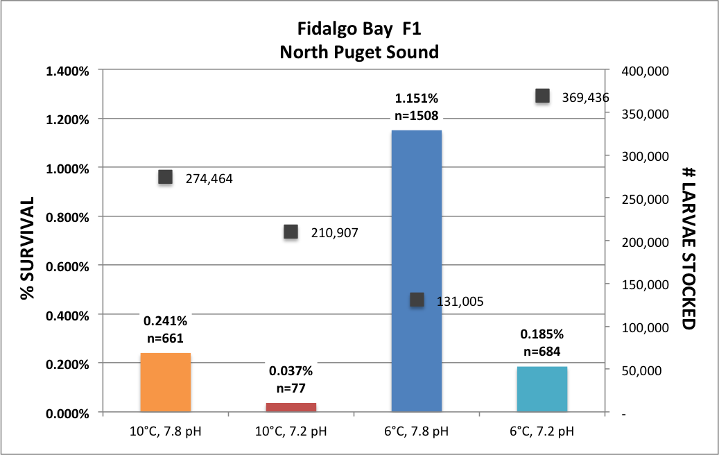
The following is data on Oly survival from larvae to juvenile. Data is adjusted for a few events where larvae were lost due to overflowed bucket, etc. Data was adjusted by calculating the mean % larvae accounted for from one bucket count to the next (pretty good, 94%), then taking the difference between the actual # counted during screening after loss event and what would be predicted by the 94% accountability rate.

I’ve been wrastling with with R to analyze my SRM data. Here’s a Jupyter notebook with initial analysis: SRM Analysis Jupyter Notebook

One of the first steps in processing SRM data is to confirm that the selected peaks actually represent the peptides, aka that our assay works. To do this, we use linear regression between PRTC retention times in DIA and SRM to calculate predicted transition RTs in collected SRM data. Then, we calculate the R^2 for PRTC and experimental peptides compared to predicted.

Before I export my data from Skyline for data analysis, I have the following final things to do:

• Adjust peak boundaries as necessary
• Remove transitions that do not align with the predicted RT. Remove any peaks that do not have at least 2 transitions.

Screened all oysters up to 450um screen, counted set on 180um silos

First steps, done on 8/8

Here’s a quick visualization of the Olympia oyster spawning data from this spring. Each chart represents a population, and within the charts data is color coded by treatment.

Setup notes

Prepping dilution curve samples

How many samples can I run?

@ 8:30am on Monday 7/24 I got my samples started again. I need to figure out how many more samples I can run within the given timeline. Here are the considerations:

• Running samples in batches of (5 samples) + (1 QC) + (1 blank) = 500 minutes total, so that’s 100 minutes / sample.
• We have until 10am on Friday 7/28
• Need 40 hrs for the dilution curve run
• So, need to be done with my samples by Wednesday 7/26 @ 6:00pm
• Time between this morning @ 8:30am when I re-started my samples & 7/26 @ 6pm = 57.5 hrs = 3450 minutes / 100 minutes/sample = 34.5 samples.
• I have 25 samples left to run, plus 2 blanks (Gblank & OBlank) which I could run twice.
• Should be done with my samples on Wednesday @ 5:30am, this includes 1 run of each blank.

Thoughts on whether or not to re-make samples

Up to this point I have 20 samples where a handful of peptides don’t show up from both PRTC and my samples. In PRTC there are 4/9 poor quality peptides, and in my samples 3/39 poor quality transitions. In an ideal world I would remake these ~20 samples, run the new batch twice while being careful with freeze/thaw and time out of the freezer. However, I don’t have time for 2 runs of remade samples. I could remake, then do 1 run of each in the hopes of capturing data on those 3 transitions. However, I think it’s best to have replicates of the 36 good quality transitions in my samples. Also, the 3 poor quality transitions were not in the sample proteins, so I can likely draw conclusions about protein quantification from the other 2 transitions. The differing rates of peptide degradation between samples does make me a little concerned; I’m wondering how folks take this into consideration.

Pro Tips for using UWPR mass spec

SPOILER ALERT The thought is that some of the peptides (in both PRTC and my samples) degrade quickly, and this is what’s causing the loss of signal. I loaded my samples in batches of 25, so samples sat out up to ~2.5 days prior to being injected. I’ll need to consider “time out of freezer” as a factor when analyzing my results. This is obvious in the dilution curve data, where PRTC total area shows an obvious decrease over time.

Readied last 25 peptide samples for mass spec

Stopped by Manchester for the AM to check on things.

Using DIA PRTC retention time data to predict SRM RT, then confirming that assays are present in my samples

Mass Spec refresher, final sample prep (+PRTC, transferring to autosampler vials)

DNR Geoduck Ctenidia Sample prep for SRM

Moved >450um seed to upwellers; combined 180um setters; standard maintenance water change, etc.

We are now running like a well oiled machine, employing progessive assembly practices.

Please see my Geoduck-DNR Repo, June Analyses folder for most up-to-date version of this process.

Happy July!

Screening day, preserved growth exp. larvae, changed growth exp water, collected new, cleaned downwellers.

Just me and Grace today, but all was very manageable.

Counted algae on broodstock manifolds, cleaned setters, SN exp. water change, new larvae, imaged growth exp.

6/28 Low impact day

• No new larvae, but NF6 Low A was “spawny”
• Water change on growth exp
• Swapped in clean banjos
• Imaged plates #1-4 from 6/26

6/29 - high impact day- screened larvae & collected new; sampled growth exp; water change, rinsed downwellers

Screened today, imaged 6/22 growth exp. & screened larvae; cleaned broodstock, yada yada yada…

Began new larval culling protcol; prepped growth exp larvae for imaging; collected new larvae; water change on growth exp.

Looked at downwellers for set, fixed growth exp. larvae from yesterday

Setters get bigger home, sampled SN growth trial, screened larvae

Trust but verify, be explicit

Screening day and more! Things went very smoothly today. Grace, Olivia and I make a good team.

Today’s vista:

6/16

Screening day.

6/13

Screening day- Arrived at 8:30am, geared up to screen through the larvae. Grace worked the screening table, Olivia managed the buckets and whatnot, I counted and re-stocked larvae, and Katie took video and images. Finished at ~2:00pm. Things went very smoothly and we got a good routine down. Here are snap-shots of the data:

Maintenance day. Steven and Beyer helped me, and it was a productive morning.

Screening day, working solo.

Tasks for the day:

• Upwelling tank:
  • Got water flowing in the upwelling tank outside, cleaned and installed connections, collected and tested hanging silos.
  • Installed immersion heater and monitored over the day
• Cleaned setting tanks
  • Inspected larvae/culch in a silo by screening through 450 onto 100; viewed under microscope for setters. Did not see any, but larvae were still present.
  • Did not screen/inspect all silos; instead, cleaned all silos, drained and cleaned setting tanks, replaced drippers & air stones.
  • Installed outflow tubing for clean drainage.
• Build freshwater adapter for manifolds. Need to run freshwater through system ASAP.
• Collected new larvae:
  • HL-6 Low
  • K-6 Low
  • K-10 Ambient
• Cleaned all K & HL broodstock fully, here’s the configuration before cleaning:

The afternoon view:

Big Screening Day. Had help from Grace, Steven, and Yaamini. Screened all larval buckets through 224 & 180um, and caught the rest on 100um. Larvae that held on 224um screen were moved to the downwelling setting tanks with microcultch at 224um. The SN & NF groups were split into two buckets, 180um and 100um (aka 180um < x <224um, and 100um < X < 180um). I did not split the HL & K groups (limited on materials and space).

From where I stand, these days:

May 29th, 2017

Here are some charts of the Oly larvae that I’ve collected & counted to date

May 23rd

Arrival Inspection

Arrival Inspection

Geoduck sample selection for next round of MS/MS

Arrived @ 9:30am

• lab meeting
  • can steal 2 HOBOs from gigas, leave 1
  • Brent suggested that it will take ~24 hrs of dual-bucket system to successfully collect only live larvae. This is a good idea, however I don’t expect there to be sufficient room - but maybe, if larval collections are staggered… ?
  • NEED TO: purchase more 5-gal buckets!
• Imaged larvae collected on 5/17, and also imaged larvae collected and saved over past week.
  • Images include triplicate samples from each collection/group (see larval collection data sheet): 1x, 2x, 3x of each on Nikon SMZ645
  • Will save to GoogleDrive, then to GitHub
• Checked catchment buckets
  • SN-10 amb B: little bit
  • NF-10 amb B: teensy amount
  • SN-10 low B: a bit
  • SN-6 amb B: little bit
  • K-10 low: some!
  • HL-10 low: maybe, probably just spermy though
  • All except HL-10 have spawned within the past 4 days, and since there is no significant amount of larvae here I will not keep them- I have a suspicion that these are from the same fertilization event, and they are trickling out of the female. Will collect for real tomorrow…
• Stole 2 HOBOs from gigas (left 1 there); downloaded the data from the HOBOs and emailed to Yaamini, then reprogrammed and launched to record T every 15 minutes, installed in broodstock buckets.
• Counted larvae collected on 5/17 & imaged larvae for size analysis later
• PSRF has agreed to collect/sample my larvae tomorrow (Friday, 5/19) while I’m on campus. I pre-labeled larval rearing buckets, got water flowing, and left instructions with Jade & Alice.
• Met with Alice to get a summary of her larval husbandry practices. PSRF hasn’t updated theirs in a couple years, and there are many lessons learned. See write-up in my GitHub (I will update as needed).
• Screened and counted larvae, imaged. Larvae went down drain today.
• Temperature is holding around 17.5

It’s been 14 full days since we moved broodstock to their separate “chambers.” From the literature, oysters release larvae on average 10-12 days after fertilization. Today I will clean all broodstock, larval catchment buckets, after which I will plan to collect larvae to save/rear.

The Avtech system allows me to download 30 days of data; I did so today, capturing pH & T data from 4/24 -> 5/16 @ ~1:30pm.

Following up on my Proteins of Interest, Part II analysis, I am taking a second, simpler look at the peak area data. This time, I am simply taking the total peak area for each protein and averaging across each treatment:

To determine over/under-expressed proteins eelgrass vs. bare treatments I did the following:

Ups and downs this weekend!

Larvae!

With demultiplexed files in Skyline I can export my results to .csv file for analysis. While I do still need to create a Retention Time Calculator and apply to data in Skyline, I’m taking an initial stab at finding differentially expressed proteins.

Olys needed a good cleaning today.

Which samples to extract next?

Checked on the spawning setup today and made some minor modifications.

Thanks to Steven & Doug for getting the Avtech probes online so we can 1) keep an eye on temp and pH remotely, and 2) download data!

For the past few weeks Olys were all housed in a 100L tank connected to a heater/chiller, which we used to increase the temp to promote gametogenesis. The goal was 1 degC per day up to 18degC, but we weren’t able to maintain that high temp due to a weak heater, and trying to keep temp high by reducing the flow rate caused the pH to drop, so that didn’t work. I’ll download HOBO temp data, but the Oly’s were kept around 14degC from 4/11 -> 5/2. This is what the setup looked like:

I’m currently importing my demultiplexed Lumos files into Skyline for the Geoduck DNR outplant study, using a .blib file that Emma generated via Pecan with all files, and the Geoduck gonad transcriptome as the database (database also has PRTC protein). Here are some screen shots of the peaks during import!

Emma ran Pecan with my geoduck samples and produced a .blib file; the next step is to run the .blib and my sample files through Skyline.

Organized the HOBO temperature data, and pulled some plots to get an initial glimpse

Just a quick update on some plumbing that needs to be done prior to getting my animals in buckets to spawn:

I prepped the histology samples taken on 4/8 and 4/13 to be sent off for slide preparation. My samples are Ostrea lurida whole visceral mass, with the goal of analyzing gonad maturation, and Yaamini’s samples are exclusively Crassostrea gigas gonad. I sampled NF, SN & HL populations on 4/8 and K populations on 4/13. Megan, Grace, Kaitlin, and Rhonda helped me by sampling the NF, SN & HL groups, and I did the K groups myself.

I’m in the midst of my first Pub-a-thon, a Roberts Lab competition. Thus far I’ve drafted methods & some background/intro language that I’ve pulled from my Oly proposal. Things have stagnated recently; it’s time to get serious. Here are the 14-day goals:

Let’s revisit the DNR geoduck mass spec data!

April 13th, 2017: Returned to Manchester solo to sample the K population (Katherine’s oysters spawned in 2015)

The next stage of the experiment is to condition my Olys in preparation for spawning. To do so, I need to get them on a system where I could gradually (1degC/day) raise the temperature of their tank from ambient (~10degC) to 18degC. Worked with Ryan Crim to figure out how best to do this:

• Condensed all Olys into one 100L tank.
• Sourced water from the ambient line that is not connected to the OA system; this line is filtered down to 5um (upon entering the hatchery). Set flow rate to 1.5 L/min.
• Set the algae dosing pump to 45 (this is the large pump that is installed on the wall). The water line is shared by Yaamini’s oysters and some spare oysters. All told, the flow rate on the line is ~6 L/min:
• Connected tank to a pump that recirculated water through the Teco TANK TK-500 1/6 HP Aquarium Chiller (also heats!).
• Set heater to 11degC (51.8degF). Instructed PSRF to increase temp to 12degC tomorrow.

April 8th, 2017: Lots of sampling today with help from the Ladies of the Roberts Lab

Megan, Rhonda, Grace, Kaitlyn, Yaamini, and myself (shoot, we forgot to take a photo, but here’s us feeding my chickens oysters. We also terminated the OA stage of this project.

Good news. We’ve actively used the OA system for 50 days with no major catastrophes. Celebrated by spending the day water sampling and cleaning oyster poop; here’s the summary:

Let’s review March goals to see how I did:

Upon arrival, pH & temp looked good, all tanks were flowing.

Yaamini & I spent the day at the hatchery cleaning and taking water chemistry. Here’s the report.

Quick morning stop @ Manchester to tend the oysters. Here’s the report.

I restarted Pecan using 1 of my geoduck .mzML files, and the full digested c. gigas proteome.

It was simple to start, and notice that I was successfully able to use the --backgroundProteome input! The concern is, as always, whether Emu has enough memory to complete all 80 isolation scheme windows for this one file. Here’s a summary:

Full day at the hatchery working solo; lots accomplished! No major surprises, except for one Pacific oyster mortality in the same tank as last week; it looked like the same oyster that appeared sickly, so while I’m not surprised, 2 morts in one tank is concerning. We will start draining/vortexing weekly, rather than bi-weekly.

Yep.

Final exam today, so Yaamini, Grace & Olivia did the daily maintenance at Manchester. Here’s what went down.

2/22-3/10: Pecan ran for nearly 3 weeks, and although it appeared to have been functioning correctly Sean discovered that there was a problem: not enough memory to save all the feature files (there should be 80 per sample; 1 per isolation window). It would simply move on to the next sample, and thus I wasn’t getting all the peptides analyzed. Check out Sean’s notebook entry for more details.

Pecan has been running since February 22nd. That’s almost 2 weeks! After several days of trying to log on to Emu to check in on the progress, I finally was able to get some information and view logs:

It’s been 21 days since the oysters started their OA treatments, and we spent the afternoon doing the standard weekly maintenance. Things are going smoothly! So far no major catastrophes, and water conditions are holding relatively steady.

Check out Yaamini’s post for details, since I wasn’t there!

Pecan! Lesson of the month: Proteomics bioinformatics is very intense.

It’s been 2 week’s since the OA experiment started, so today was an intensive cleaning and re-organizing day. But first, Yaamini and I spent the morning at the monthly hatchery meeting, and learning about how Olympia oysters swim around in OA from Western Washigton crew (Shawn Arellano and her students). Then…

Here’s my laundry list. Obviously, I like bullets:

Here’s a quick look at the continuous temperature data. Notice the tight cycling in the “cold” treatment due to the chiller, and the slower, diurnal cycling in the “ambient” (aka warm!) group:

We check on our oysters every Monday and Wednesday. Mondays are minimum effort days, where we clean filters, collect water chemistry samples and measurements, clean algae lines with bleach, and make sure everything is flowing and pH/T are stable. Yaamini and I are dividing duties, so I’ll post links to her notebook when she goes out and I don’t.

Yaamini and I spent the afternoon with our oysters.

Popped into Manchester a couple mornings to take water chemistry.

Got the oysters into pH treatments today! This, after a couple surprises…

Spent the day @ Manchester making the final (hopefully) touches to OA system. Also sampled the F2 population (Katherine’s). Here’s a breakdown:

Header Tanks:

• Header 2, which was supposed to be ambient, was consistently reading ~7.5. This is too low, since ambient in other tanks have been reading 7.78. I disconnected the CO2 tube from the manchurian injector, and capped it. I drained the tank 1/2 way, and refilled. pH levelled off to 7.78 by the end of the day in the header (H2).
• After watching the pH in Header 1 since Wednesday, and seeing pH drop to low 6, it was obvious that adjustments were needed to the CO2 injections system. Here’s what I did:
  • Drained Header 1 to 1/3 the volume, and refilled
  • Lowered pressure in main CO2 line to ~15psi
  • Increased the injection frequency from 120 to 180 seconds
  • Decreased the injection duration from 0.8 to 0.4 seconds
  • Changed set point to 7.38 <-> 7.42; since Ambient is ~7.8, I want a larger difference between treatments
  • Note: I noticed water had collected again in H1’s CO2 line. I drained it again; perhaps we need a better sealant on the CO2 connection.
• It’s been ~18hrs since making htese adjustments and pH seems to be hovering around 7.4! Will continue to monitor.
• Reminders:
  • Header 1 is connected to Relay 2 for CO2 injection
  • Yellow Durafet outputs to the left Honeywell screen, top, as “input pv 1”
  • PInk Durafet outputs to the left Honeywell screen, bottom, as “input pv 2”
  • Green Durafet ouputs to the right Honeywell screen, bottom, as “input pv 2”

Culture Tanks:

• Drained all tanks, cleaned with Vortex.
• One tank has outflow drain @ bottom; capped that.
  • Note: late in the day I saw 2 nicely insulated tanks from last year’s experiment stored in the Warehouse. Let’s use these next time we clean tanks * Labeled tanks: #1-3 = low pH #4-6 = ambient
• Labeled and installed HOBO temperature loggers - one logger per tank.
• Set flow rate on all tanks to 1 Liter/minute. Did not mark valves to replicate this at each cleaning - will do so next time.

Oysters are set to go into pH treatments (ambient, 7.5) on Wedneday 2/8, so on Sunday I went to Manchester to get the OA system running, so we could test the CO2 injectors and Durafets.

Full day of sampling! THANK YOU to Grace for materials prep, Megan Hintz, Olivia & Lindsay Alma for helping Yaamini and me with the sampling, and to Steven for the oversight and OA system prep.

We went out to Manchester on 1/25/2017 to check on the Olympia oysters that are already (!) undergoing temperature treatment, to assess the OA system.

Check it out! This is a screen shot of the Lumos mass spec collecting data on my geoduck samples’ peptide contents. The most important track to monitor is the top track, which is the System Pressure (psi). The long plateus correspond to the samples’ peptides being run, short plateus (I believe) correspond to cleaning between samples.

Met Emma at the UWPR in South Lake Union; she brought our samples & the acetonitrile that we used for our samples.
We transferred our samples into labeled autosampler vials. NOTE: next time we need to bring empty autosampler vials for our blanks!!!

There were a few last items that needed to happen prior to injecting samples into Mass Spec. Here they are!

January 2017 Goals

The finale: a day of desalting

Evaporating - that’s it!

Making peptides via Mini-Trypsin Digestion

Today I determined the concentration of proteins in my samples. This was done via the Thermo Scientific - 23225 - BCA PROTEIN ASSAY KIT, following the protein prep protocol and Rhonda Elliott’s recent lab notebook entry.

Today’s lab work involved homogenizing the tissue in solution, then sonicating to lyse the cells.

DNR Geoduck OA overview

After a couple months of school under my belt, here is a list of non-class related items I’d like to accomplish by December:

This is a draft research plan for a project I could execute starting winter 2016/2017.

This is a draft research plan for a project I could possibly execute winter 2016/2017. I invite any and all feedback. Thanks!

Last week I shadowed Hollie while she performed the first few steps of DNA extraction. Here’s what I learned about the process and general tips for working in that lab:

Ok, now let’s play the shell game!